Logarithmic Functions as Models of Proportional Growth
Logarithmic functions are the inverse functions of exponential functions and are used to model situations involving proportional growth or repeated multiplication.
In these situations, the input values change proportionally over equal-length output-value intervals. This reverses the behavior of exponential functions, where output values change proportionally over equal-length input intervals.
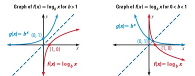
For a logarithmic function in general form
\( \mathrm{ \displaystyle f(x)=\log_b x } \)
the output value represents the number of times the initial value has been multiplied by the base.
In particular, when the output value is a whole number, it indicates how many factors of the base are needed to reach the input value:
\( \mathrm{ \displaystyle \log_b x = n \iff b^n = x } \)
Key Interpretation
• Exponential models describe how much a quantity grows
• Logarithmic models describe how many multiplicative steps occurred
Example
A quantity grows by repeatedly multiplying by 3. Determine how many multiplications are needed to reach a value of 81.
▶️ Answer/Explanation
Model the situation using a logarithmic function:
\( \mathrm{ \displaystyle \log_3 81 } \)
Rewrite in exponential form:
\( \mathrm{ \displaystyle 3^n=81 } \)
Since \( \mathrm{3^4=81} \),
\( \mathrm{ \displaystyle \log_3 81=4 } \)
Conclusion
The quantity was multiplied by 3 a total of 4 times.
Example
A bacterial culture doubles repeatedly. The population reaches 64 times its initial size. Use a logarithmic model to determine how many doubling periods have occurred.
▶️ Answer/Explanation
Doubling corresponds to a base of 2:
\( \mathrm{ \displaystyle \log_2 64 } \)
Rewrite in exponential form:
\( \mathrm{ \displaystyle 2^n=64 } \)
Since \( \mathrm{2^6=64} \),
\( \mathrm{ \displaystyle \log_2 64=6 } \)
Conclusion
The population doubled 6 times to reach 64 times its original size.
Constructing Logarithmic Function Models Using Transformations
Logarithmic function models can be constructed by applying transformations to the parent logarithmic function
\( \mathrm{ \displaystyle f(x)=a\log_b x } \)
These transformations are chosen based on the characteristics of a context or data set, such as shifts in starting values, scaling of outputs, or horizontal translations.
A general transformed logarithmic model can be written as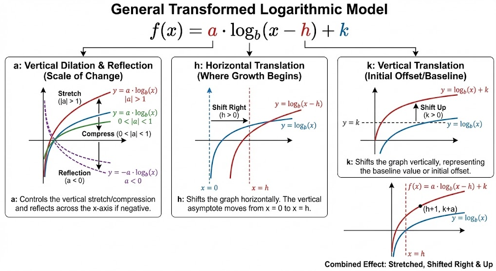
\( \mathrm{ \displaystyle f(x)=a\log_b(x-h)+k } \)
where each parameter has a modeling interpretation:
• \( \mathrm{a} \): vertical dilation and possible reflection, matching the scale of change
• \( \mathrm{h} \): horizontal translation, adjusting where growth begins
• \( \mathrm{k} \): vertical translation, representing an initial offset or baseline value
By selecting appropriate values of \( \mathrm{a} \), \( \mathrm{h} \), and \( \mathrm{k} \), the logarithmic model can closely represent real-world data.
Example
A sound intensity model follows a logarithmic pattern and has a baseline value of 30 when \( \mathrm{x=1} \). The intensity increases slowly as \( \mathrm{x} \) increases.
Construct a suitable logarithmic model.
▶️ Answer/Explanation
Start with the parent function \( \mathrm{\log_{10} x} \).
Since the baseline is 30 at \( \mathrm{x=1} \), add 30:
\( \mathrm{ \displaystyle f(x)=\log_{10}x+30 } \)
Conclusion
The logarithmic model is \( \mathrm{f(x)=\log_{10}x+30} \).
Example
A data set shows logarithmic behavior that begins only after \( \mathrm{x=5} \), and the output values are twice as large as those of the parent function.
Construct a logarithmic model using base 2.
▶️ Answer/Explanation
Start with the parent function \( \mathrm{\log_2 x} \).
Shift the graph right by 5 units:
\( \mathrm{ \displaystyle \log_2(x-5) } \)
Apply a vertical stretch by a factor of 2:
\( \mathrm{ \displaystyle f(x)=2\log_2(x-5) } \)
Conclusion
The logarithmic model is \( \mathrm{f(x)=2\log_2(x-5)} \).
Logarithmic Regression Models
When a data set shows a pattern where output values increase or decrease slowly while input values grow proportionally, a logarithmic function model may be appropriate.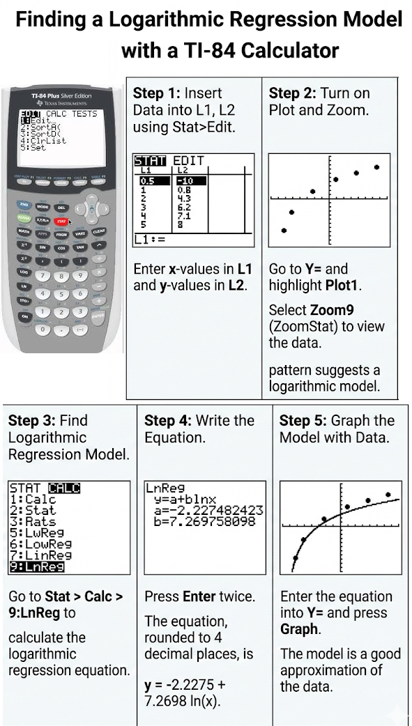
In such cases, a logarithmic model can be constructed using technology through a process called logarithmic regression.
Logarithmic regression determines the constants that best fit the data in a model of the form
\( \mathrm{ \displaystyle f(x)=a\log_b x + k } \)
The regression minimizes the overall error between the observed data values and the values predicted by the logarithmic model.
This method is commonly used when:
• The rate of change decreases as input values increase
• The graph rises or falls quickly at first and then levels off
• Residuals show no clear pattern when a logarithmic model is used
Example
A data set relates the number of practice hours to performance score. The scores increase rapidly at first and then increase more slowly.
A logarithmic regression using technology gives the model
\( \mathrm{ \displaystyle f(x)=12\log_{10}x+45 } \)
Interpret the model.
▶️ Answer/Explanation
The logarithmic form indicates diminishing returns as practice hours increase.
The constant 45 represents a baseline performance score, and the coefficient 12 scales the growth.
Conclusion
The model suggests that early practice leads to large improvements, while later practice leads to smaller gains.
Example
A scientist records the brightness of a star relative to distance. A logarithmic regression produces the model
\( \mathrm{ \displaystyle f(x)=-5\log_{10}x+20 } \)
Explain why a logarithmic model is reasonable.
▶️ Answer/Explanation
As distance increases proportionally, brightness decreases by smaller and smaller amounts.
The negative coefficient reflects the decreasing trend.
Conclusion
The logarithmic regression appropriately captures the slow rate of change at large distances.
The Natural Logarithm Function in Real-World Modeling
The natural logarithm function is commonly used to model real-world phenomena in which growth or decay occurs continuously.
The natural logarithm is defined as the logarithm with base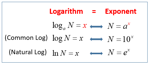
\( \mathrm{ \displaystyle e \approx 2.718 } \)
and is written as
\( \mathrm{ \displaystyle f(x)=\ln x } \)
Natural logarithms arise naturally as the inverse of exponential functions of the form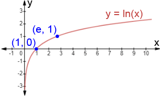
\( \mathrm{ \displaystyle g(x)=e^x } \)
They are especially useful when:
• growth or decay occurs continuously rather than in discrete steps
• input values change proportionally while output values change by equal amounts
• the model involves rates of change related to the current amount
Common applications include population growth, radioactive decay, cooling processes, economics, and natural sciences.
Example
A population grows continuously according to an exponential model. The time required for the population to reach a certain size is needed.
Explain why a natural logarithm model is appropriate.
▶️ Answer/Explanation
Exponential population models use base \( \mathrm{e} \) to represent continuous growth.
Solving for time requires applying the inverse of the exponential function, which is the natural logarithm.
Conclusion
Natural logarithms are appropriate because they reverse continuous exponential growth.
Example
The temperature of an object decreases continuously as it cools. The relationship between temperature and time follows an exponential decay pattern.
Explain how the natural logarithm is used in analyzing this situation.
▶️ Answer/Explanation
Cooling processes involve continuous decay modeled by exponential functions with base \( \mathrm{e} \).
Taking the natural logarithm allows time to be isolated and interpreted.
Conclusion
The natural logarithm provides a practical way to analyze and interpret continuous decay phenomena.