Semi-Log Plots and Exponential Behavior
A semi-log plot is a graph in which one axis is scaled logarithmically while the other axis remains on a standard linear scale.
When the y-axis is logarithmically scaled and the x-axis is linear, functions or data sets that demonstrate exponential behavior appear as straight lines.
This occurs because exponential functions have the form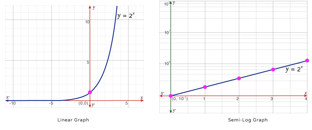
\( \mathrm{ \displaystyle y=ab^x } \)
Taking the logarithm of the output gives
\( \mathrm{ \displaystyle \log y=\log a + x\log b } \)
This equation is linear in \( \mathrm{x} \), which explains why exponential data form a straight line on a semi-log plot.
Key Interpretation
• Straight line on a semi-log plot ⇒ exponential relationship
• Slope represents the growth or decay factor
• Intercept relates to the initial value
Example
A population follows the model
\( \mathrm{ \displaystyle y=500(1.2)^x } \)
Explain how this model would appear on a semi-log plot with a logarithmic y-axis.
▶️ Answer/Explanation
Taking logarithms gives
\( \mathrm{ \displaystyle \log y=\log 500 + x\log 1.2 } \)
This is a linear equation in \( \mathrm{x} \), so the graph appears as a straight line on the semi-log plot.
Conclusion
The straight-line pattern confirms exponential growth.
Example
A data set appears curved on a standard graph but forms a straight line when plotted on a semi-log plot with a logarithmic y-axis.
What does this indicate about the relationship between the variables?
▶️ Answer/Explanation
A straight line on a semi-log plot indicates that the logarithm of the output changes linearly with the input.
Conclusion
The variables have an exponential relationship.
Applying Linear Modeling Techniques to Semi-Log Graphs
A key advantage of semi-log graphs is that techniques used to model linear functions can be directly applied when analyzing exponential data.
When the y-axis is logarithmically scaled, an exponential relationship of the form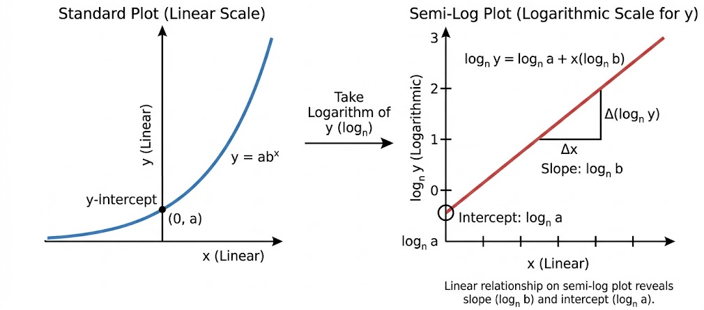
\( \mathrm{ \displaystyle y=ab^x } \)
appears as a straight line on the semi-log graph because
\( \mathrm{ \displaystyle \log y=\log a + x\log b } \)
This linear relationship allows the same methods used for linear models to be applied, including:
• estimating slope using two points
• interpreting slope as a rate of change
• using linear regression and residual plots
In this context, the slope of the line represents the logarithm of the growth or decay factor, and the intercept relates to the initial value.
Example
A data set appears as a straight line on a semi-log plot with a logarithmic y-axis.
Explain how the slope of the line is interpreted.
▶️ Answer/Explanation
Because the graph is linear on a semi-log plot, the slope can be found using two points, just as in linear modeling.
The slope represents \( \mathrm{\log b} \), where \( \mathrm{b} \) is the exponential growth or decay factor.
Conclusion
A constant slope on a semi-log plot indicates a constant multiplicative rate of change.
Example
A researcher fits a straight line to data on a semi-log plot and finds no visible pattern in the residuals.
What does this indicate about the model?
▶️ Answer/Explanation
A residual plot with no pattern indicates that the linear fit on the semi-log graph is appropriate.
This confirms that the original data follow an exponential model.
Conclusion
Linear modeling techniques validate exponential relationships when applied to semi-log graphs.
Linear Models from Exponential Functions on Semi-Log Plots
An exponential model of the form
\( \mathrm{ \displaystyle y=ab^x } \)
can be rewritten as a linear model when the dependent variable is plotted on a logarithmic scale.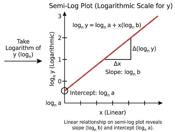
Taking the logarithm with base \( \mathrm{n} \), where \( \mathrm{n>0} \) and \( \mathrm{n\ne1} \), gives
\( \mathrm{ \displaystyle \log_n y=\log_n a + x\log_n b } \)
On a semi-log plot, this relationship appears as a straight line with:
• linear rate of change (slope): \( \mathrm{\log_n b} \)
• initial linear value (intercept): \( \mathrm{\log_n a} \)
Thus, exponential growth or decay in the original model corresponds to a constant slope in the semi-log representation.
Example
Given the exponential model
\( \mathrm{ \displaystyle y=200(1.5)^x } \)
write the corresponding linear model for a semi-log plot using base 10.
▶️ Answer/Explanation
Take the logarithm base 10 of both sides:
\( \mathrm{ \displaystyle \log_{10} y=\log_{10}200 + x\log_{10}1.5 } \)
This is a linear equation of the form \( \mathrm{y=mx+c} \) on the semi-log plot.
Conclusion
The slope is \( \mathrm{\log_{10}1.5} \), and the intercept is \( \mathrm{\log_{10}200} \).
Example
A straight line on a semi-log plot has slope \( \mathrm{\log_{10}2} \) and intercept \( \mathrm{\log_{10}50} \).
Determine the corresponding exponential model.
▶️ Answer/Explanation
From the linear form:
\( \mathrm{ \displaystyle \log_{10} y=(\log_{10}2)x+\log_{10}50 } \)
Rewrite in exponential form:
\( \mathrm{ \displaystyle y=50\cdot2^x } \)
Conclusion
The exponential model has initial value 50 and growth factor 2.