AP Precalculus -2.3 Exponential Functions- FRQ Exam Style Questions - Effective Fall 2023

AP Precalculus -2.3 Exponential Functions- FRQ Exam Style Questions – Effective Fall 2023

AP Precalculus -2.3 Exponential Functions- FRQ Exam Style Questions – AP Precalculus- per latest AP Precalculus Syllabus.

AP Precalculus – FRQ Exam Style Questions- All Topics

Question

The Chinese bamboo tree exhibits a unique growth pattern. Once a seed has been planted, the Chinese bamboo tree does not break through the ground for several years. However, once it breaks through the ground, the Chinese bamboo tree grows exponentially. In one particular experiment, a group of biologists recorded the height of a Chinese bamboo tree once it broke through the ground. After one week ($t = 1$), the Chinese bamboo tree measured 3 feet, and after five weeks ($t = 5$), the same tree measured 89 feet.

The height of the Chinese bamboo tree can be modeled by the function $H$ given by $H(t) = ab^x$, where $H(t)$ is the height of the tree, in feet, $t$ weeks after it first breaks ground.

(A) (i) Use the given data to write two equations that can be used to find the values for constants $a$ and $b$ in the expression for $H(t)$.

(ii) Find the values for $a$ and $b$.

(B) (i) Use the given data to find the average rate of change of the height of the Chinese bamboo tree, in feet per week, from $t = 1$ to $t = 5$ weeks. Express your answer as a decimal approximation. Show the computations that lead to your answer.

(ii) Interpret the meaning of your answer from (i) in the context of the problem.

(iii) Consider the average rates of change of $H$ from $t = 5$ to $t = p$ weeks, where $p > 5$. Are these average rates of change less than or greater than the average rate of change from $t = 1$ to $t = 5$ weeks found in (i)? Explain your reasoning.

(C) For which $t$-value, $t = 4$ weeks or $t = 11$ weeks, should the biologists have more confidence in when using the model $H$? Give a reason for your answer in the context of the problem.

Most-appropriate topic codes (AP Precalculus CED):

• 2.5: Exponential Function Context and Data Modeling – part A
• 1.2: Rates of Change – part B(i), B(ii)
• 2.3: Exponential Functions – part B(iii)
• 1.13: Function Model Selection and Assumption Articulation – part C

▶️ Answer/Explanation

Detailed solution

(A)(i) Equations
Substituting the points $(1, 3)$ and $(5, 89)$ into $H(t) = ab^t$:
1. $3 = ab^1$ (or $3 = ab$)
2. $89 = ab^5$

(A)(ii) Values for a and b
Dividing equation 2 by equation 1: $\frac{ab^5}{ab} = \frac{89}{3} \implies b^4 = 29.67$.
Solving for $b$: $b = (29.67)^{0.25} \approx 2.33$.
Solving for $a$: $a = \frac{3}{2.33} \approx 1.29$.

(B)(i) Average Rate of Change
$\text{Rate} = \frac{H(5) – H(1)}{5 – 1} = \frac{89 – 3}{4} = \frac{86}{4} = 21.5$
Answer: 21.5 feet per week.

(B)(ii) Interpretation
The answer indicates that between the first and fifth weeks, the bamboo tree grew at an average speed of 21.5 feet per week.

(B)(iii) Comparison
Greater. The function represents exponential growth ($b > 1$), which is concave up. This means the rate of growth increases over time, so the rate after week 5 will be steeper than the rate before week 5.

(C) Confidence
$t = 4$ weeks.
The biologists should be more confident in $t=4$ because it is an interpolation (within the observed data range). $t=11$ is an extrapolation; biological growth cannot remain exponential indefinitely, so the model is likely inaccurate that far out.

Question

A dog food bowl has a certain number of dog food pellets. A dog eats a fraction of the remaining food per minute. At $t = 1$ minute, 145 pellets are left; at $t = 2$ minutes, 115 pellets are left. The situation is modeled by $P(t) = ae^{bt}$, where $P(t)$ is the number of pellets left after $t$ minutes.

(A) Find an exponential function that models this situation.
(B) (i) Find the average rate of change from $t = 0$ to $t = 4$. Explain its meaning.
(ii) Will the average rate of change from $t = 4$ to $t = t_a$ (with $t_a > 4$) be greater or less than that from $t = 0$ to $t = 4$? Justify.
(C) As $t \to \infty$, does the model make sense contextually? Why or why not?

Most-appropriate topic codes (AP Precalculus CED):

• 2.5: Exponential Function Context and Data Modeling – part (A), part (C)
• 1.2: Rates of Change – part (B)(i), (B)(ii)
• 2.3: Exponential Functions – part (B)(ii)
• 3.2: Apply numerical results in a given mathematical or applied context – part (B)(i), (C)
• 3.3: Support conclusions or choices with a logical rationale or appropriate data – part (B)(ii), (C)

▶️ Answer/Explanation

Detailed solution

(A) Exponential model $P(t) = ae^{bt}$

Given: $P(1) = 145$, $P(2) = 115$.
Divide the equations: $\frac{P(2)}{P(1)} = \frac{115}{145} = \frac{23}{29} \approx 0.7931 = e^{b(2-1)} = e^b$.
So $b = \ln\left(\frac{23}{29}\right) \approx \ln(0.7931) \approx -0.2318$.
Use $P(1) = ae^{b\cdot1} = 145$: $a = 145 \cdot e^{-b} = 145 \cdot \frac{29}{23} \approx 145 \cdot 1.2609 \approx 182.83$.
Alternatively, compute directly: $a = P(1) e^{-b} = 145 \cdot \frac{29}{23} = \frac{145 \cdot 29}{23} = \frac{4205}{23} \approx 182.826$.
Thus, $P(t) \approx 182.826 e^{-0.2318 t}$.

(B) i. Average rate of change from $t = 0$ to $t = 4$

$P(0) = a \approx 182.826$.
$P(4) = 182.826 e^{-0.2318 \cdot 4} \approx 182.826 e^{-0.9272} \approx 182.826 \cdot 0.3956 \approx 72.34$.
Average rate = $\frac{P(4) – P(0)}{4 – 0} \approx \frac{72.34 – 182.826}{4} = \frac{-110.486}{4} \approx -27.622$ pellets per minute.
Meaning: On average over the first 4 minutes, the dog ate about 27.6 pellets per minute.

(B) ii. Comparison of average rates

For an exponential decay $P(t) = ae^{bt}$ with $b < 0$, the function is decreasing and concave up (since $P”(t) = ab^2 e^{bt} > 0$).
In a concave up decreasing function, the average rate of change over an interval decreases in magnitude (becomes less negative) as the interval moves to the right.
Thus, the average rate from $t = 4$ to $t = t_a$ will be greater (less negative) than that from $t = 0$ to $t = 4$.
Reason: The instantaneous rate (derivative) is negative but increasing (becoming less negative), so later intervals have a smaller rate of loss.

(C) Limit as $t \to \infty$

$\lim_{t \to \infty} P(t) = \lim_{t \to \infty} ae^{bt} = 0$ because $b < 0$.
Context: The model predicts the pellets approach zero but never actually reach it. In reality, the dog will finish all pellets in finite time, so the model is not perfectly accurate for very large $t$. However, it is a good approximation for the decay process while pellets remain.
Thus, the model does not fully make sense as $t \to \infty$ because it predicts the dog never finishes, while in reality the bowl becomes empty at some finite time.

Question

An increasing, continuous function $g(x)$ has outputs of some values of $x$ shown in the table. $f(x)$ is a function shown to the right as the graph.

(A) (i) Estimate the value of $g(f^{-1}(1))$ for all values if it is defined.
(ii) If $h(x) = \frac{g(x)}{f(x)}$, then define any discontinuities, their type, and their location when $x > 0$.
(B) Suppose $j(x) = \frac{1}{4.998} \ln(x) \cdot e^{2\sin(\sqrt{x})}$ could be used to model $f(x)$.
(i) Determine the end behavior of $j$ when $x$ increases without bound.Express your answer with the mathematical definition of a limit if it exists. If it does not exist, explain why.
(ii) Determine the vertical asymptote of $j$ when $x$ approaches 0 from the right.Express your answer with the mathematical definition of a limit if it exists. If it does not, explain why.
(C) Determine if $g(x)$, using the values in the table, can be best modeled with a linear, quadratic, exponential, or logarithmic function. Explain your answer based on the relationship between the change
in the output values of 𝑔 and the change in the input values of 𝑔.

Most-appropriate topic codes (AP Precalculus CED):

• 1.9: Rational Functions and Vertical Asymptotes – part A(ii)
• 2.3: Exponential Functions – part B(i), B(ii)
• 2.8: Inverse Functions – part A(i)
• 2.11: Logarithmic Functions – part B(i), B(ii), C
• 2.14: Logarithmic Function Context and Data Modeling – part C

▶️ Answer/Explanation

Detailed solution

(A) i. $g(f^{-1}(1))$

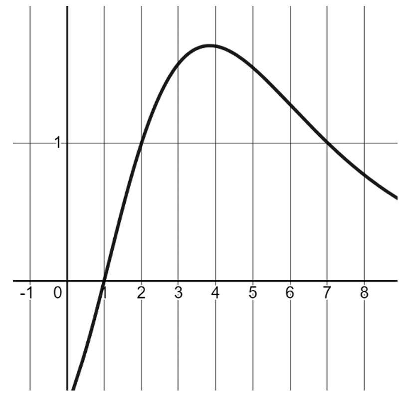
From the graph of $f(x)$, $f^{-1}(1)$ means find $x$ such that $f(x) = 1$.
From the graph, $f(x) = 1$ at approximately $x \approx 2.5$. So $f^{-1}(1) \approx 2.5$.
From the table, $g(2) = 1$, $g(4) = 2$. Since $g$ is increasing and continuous, by linear interpolation for $x \approx 2.5$: $g(2.5) \approx 1 + \frac{2.5-2}{4-2} \cdot (2-1) = 1 + 0.25 = 1.25$.
Thus, $g(f^{-1}(1)) \approx 1.25$.

(A) ii. $h(x) = \frac{g(x)}{f(x)}$, $x > 0$

Discontinuities occur where $f(x) = 0$ or where $f$ is undefined (but $f$ appears continuous from the graph for $x>0$).
From the graph, $f(x) = 0$ at $x \approx 1.5$ (where graph crosses x-axis). That is the only zero of $f$ for $x>0$.
At $x \approx 1.5$, $g(x) \neq 0$ (since $g$ is about 0.5 between $g(1)=0$ and $g(2)=1$).
Thus, $h(x)$ has a vertical asymptote at $x \approx 1.5$ because denominator → 0, numerator nonzero → $h(x) \to \pm\infty$.
Type: infinite discontinuity (vertical asymptote).

(B) i. End behavior of $j(x) = \frac{1}{4.998} \ln(x) \cdot e^{2\sin(\sqrt{x})}$ as $x \to \infty$

As $x \to \infty$, $\ln(x) \to \infty$.
The factor $e^{2\sin(\sqrt{x})}$ oscillates between $e^{-2}$ and $e^{2}$ because $\sin(\sqrt{x})$ oscillates in $[-1,1]$.
Thus $j(x)$ oscillates with amplitude growing like $\ln(x)$. The limit does not exist because oscillations persist and amplitude grows without bound.
Limit expression: $\lim_{x \to \infty} j(x)$ does not exist.

(B) ii. Vertical asymptote as $x \to 0^+$

As $x \to 0^+$, $\ln(x) \to -\infty$.
The factor $e^{2\sin(\sqrt{x})} \to e^{0} = 1$ (since $\sqrt{x} \to 0$, $\sin(\sqrt{x}) \to 0$).
Thus $j(x) \to -\infty$.
Limit expression: $\lim_{x \to 0^+} j(x) = -\infty$. So vertical asymptote at $x=0$.

(C) Best model for $g(x)$ from the table:

Check changes in $g(x)$ as $x$ doubles:
From $x=0.5$ to $x=1$, $\Delta g = 1$.
From $x=1$ to $x=2$, $\Delta g = 1$.
From $x=2$ to $x=4$, $\Delta g = 1$.
From $x=4$ to $x=8$, $\Delta g = 1$.
Each time $x$ doubles, $g(x)$ increases by about 1. This suggests a logarithmic relationship: $g(x) \approx a + b \ln(x)$.
Thus, $g(x)$ is best modeled by a logarithmic function.

Question

The figure shows the graph of the function $ f $ on its domain of $ -3.5 \le x \le 3.5 $. The points $ (-3,1) $, $ (0,1) $, and $ (3,1) $ are on the graph of $ f $. The function $ g $ is given by $ g(x)=2.916\cdot(0.7)^x $.

(A)
(i) The function $ h $ is defined by $ h(x)=(g\circ f)(x)=g(f(x)) $. Find the value of $ h(3) $ as a decimal approximation, or indicate that it is not defined.
(ii) Find all values of $ x $ for which $ f(x)=1 $, or indicate that there are no such values.

(B)
(i) Find all values of $ x $, as decimal approximations, for which $ g(x)=2 $, or indicate that there are no such values.
(ii) Determine the end behavior of $ g $ as $ x $ increases without bound. Express your answer using the mathematical notation of a limit.

(C)
(i) Determine if $ f $ has an inverse function.
(ii) Give a reason for your answer based on the definition of a function and the graph of $ y=f(x) $.

Most-appropriate topic codes (CED):

• TOPIC 1.7: Composition of Functions — part (A)
• TOPIC 2.3: Exponential Functions — part (B)
• TOPIC 1.5: Inverse Functions — part (C)

▶️ Answer/Explanation

Concise solution

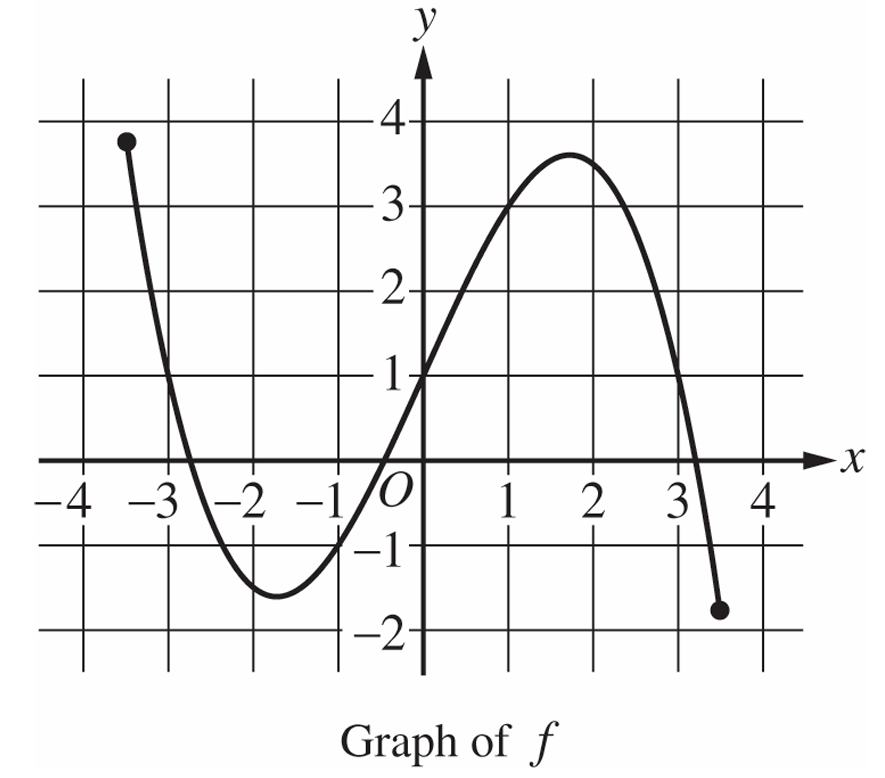
(A)(i)
From the graph, $ f(3)=1 $.
$ h(3)=g(f(3))=g(1)=2.916(0.7)=2.041 $.

(A)(ii)
From the graph, $ f(x)=1 $ at $ x=-3,0,3 $.

(B)(i)
$ 2.916(0.7)^x=2 $
$ (0.7)^x=\frac{2}{2.916} $
Taking logarithms,
$ x=\frac{\ln(\frac{2}{2.916})}{\ln(0.7)}\approx1.057 $.

(B)(ii)
Since $ 0.7<1 $, $ (0.7)^x \to 0 $ as $ x \to \infty $.
$ \lim_{x\to\infty} g(x)=0 $.

(C)
$ f $ does not have an inverse because it is not one-to-one.
For example, $ f(-3)=f(0)=f(3)=1 $.

Question

A student won $500$ in an art contest. At first, the student kept the money in a desk. After $10$ months, the student deposited the money in a savings account that earned interest. Six months after depositing the money ($t = 6$), the amount in the account is $508.67$. Twelve months after depositing the money ($t = 12$), the amount in the account is $517.50$.

The amount of money the student has can be modeled by the piecewise function $M$ given by: $$M(t) = \begin{cases} 500 & \text{for } -10 \le t < 0 \\ ab^{(t/12)} & \text{for } t \ge 0 \end{cases}$$ where $M(t)$ is the amount, in dollars, at time $t$ months since the $500$ was deposited into the savings account. A negative value for $t$ represents the number of months before the student deposited the $500$ into the savings account.

Part A

(i) Use the given data to write two equations that can be used to find the values for constants $a$ and $b$ in the expression for $M(t)$.

(ii) Find the values for $a$ and $b$ as decimal approximations.

Part B

(i) Use the given data to find the average rate of change of the amount of money the student has, in dollars per month, from $t = -2$ to $t = 12$ months. Express your answer as a decimal approximation. Show the computations that lead to your answer.

(ii) Use $M(12)$ and the average rate of change found in (i) to estimate the amount of money, in dollars, the student has when $t = 20$ months. Show the work that leads to your answer.

(iii) Let $A(t)$ be the estimate of the amount of money, in dollars, the student has at time $t$ months using the average rate of change found in (i). If $A(t)$ is used to estimate values for $M(t)$ for $t > 12$, the error in the estimates will increase as $t$ increases. Explain why this is true.

Part C

The student plans to close the account when the amount of money in the account reaches $565$. Explain how this information can be used to determine the domain limitations for the model $M$.

▶️ Answer/Explanation

Detailed solution

Part A

(i)
Using the data $M(6) = 508.67$ and $M(12) = 517.50$:
$ab^{(6/12)} = 508.67$ (or $ab^{0.5} = 508.67$)
$ab^{(12/12)} = 517.50$ (or $ab = 517.50$)

(ii)
Divide the second equation by the first: $\frac{ab}{ab^{0.5}} = \frac{517.50}{508.67}$
$b^{0.5} \approx 1.017359…$
$b \approx (1.017359…)^2 \approx 1.035019…$
Using $ab = 517.50 \implies a = \frac{517.50}{1.035019…} \approx 500$
Final values: $a \approx 500.00$ and $b \approx 1.035$

Part B

(i)
$t = -2$ falls in the interval $-10 \le t < 0$, so $M(-2) = 500$.
$t = 12$ is given as $M(12) = 517.50$.
Average Rate of Change $= \frac{M(12) – M(-2)}{12 – (-2)}$
$= \frac{517.50 – 500}{12 + 2}$
$= \frac{17.50}{14} = 1.25$ dollars per month.

(ii)
The linear estimate $A(t)$ uses the point $(12, 517.50)$ and slope $1.25$.
$A(20) = M(12) + 1.25(20 – 12)$
$A(20) = 517.50 + 1.25(8)$
$A(20) = 517.50 + 10 = 527.50$ dollars.

(iii)
The model $M(t)$ for $t \ge 0$ is an exponential function ($b > 1$), which is concave up.
The estimate $A(t)$ is a linear function (a secant line).
Since $M(t)$ is increasing at an increasing rate (exponential growth), the linear model will fall further behind the actual values as $t$ increases.

Part C

The model is only valid as long as the account is open.
Setting $M(t) = 565$ allows us to solve for the maximum value of $t$.
$500(1.035)^{(t/12)} = 565$
This value of $t$ serves as the upper bound (maximum) for the domain of the model $M$.

AP Precalculus -2.3 Exponential Functions- FRQ Exam Style Questions - Effective Fall 2023