Home / AP® Exam / AP® PreCalculus / AP® Precalculus

AP Precalculus -2.5 Exponential Function Modeling- Study Notes - Effective Fall 2023

AP Precalculus -2.5 Exponential Function Modeling- Study Notes – Effective Fall 2023

AP Precalculus -2.5 Exponential Function Modeling- Study Notes – AP Precalculus- per latest AP Precalculus Syllabus.

LEARNING OBJECTIVE

Construct a model for situations involving proportional output values over equal-length input-value intervals.
Apply exponential models to answer questions about a data set or contextual scenario.

Key Concepts: 

  • Exponential Functions as Models of Growth

  • Revealing Proportional Growth Using an Additive Constant

  • Constructing an Exponential Function Model

  • Constructing Exponential Models Using Transformations

  • Exponential Regression Using Technology

  • The Natural Base  in Exponential Models

  • Interpreting the Base of an Exponential Model

  • Equivalent Forms of Exponential Functions

  • Using Exponential Models for Prediction

AP Precalculus -Concise Summary Notes- All Topics

Exponential Functions as Models of Growth

Exponential functions are commonly used to model growth patterns in which output values change proportionally over equal-length input-value intervals.

This proportional behavior means that for a fixed interval length \( \mathrm{h} \),

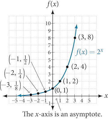
\( \mathrm{ \displaystyle \dfrac{f(x+h)}{f(x)} = \text{constant} } \)

for all values of \( \mathrm{x} \).

When the input values are whole numbers, exponential functions model situations involving repeated multiplication of a constant factor applied to an initial value.

In general, an exponential function can be written as

\( \mathrm{ \displaystyle f(x) = ab^x } \)

where \( \mathrm{a} \) is the initial value and \( \mathrm{b} \) is the constant multiplier applied at each step.

This makes exponential functions ideal for modeling population growth, compound interest, and repeated percent increase or decrease.

Example

A quantity starts at 100 and increases by 20% each time period.

Write an exponential model for the situation.

▶️ Answer/Explanation

The initial value is \( \mathrm{a = 100} \).

An increase of 20% corresponds to a multiplier of \( \mathrm{1.2} \).

\( \mathrm{ \displaystyle f(x) = 100(1.2)^x } \)

Conclusion

Each increase of 1 in the input multiplies the output by 1.2.

Example

The value of a car is initially \$20,000 and decreases by 15% each year.

Write an exponential model for the value of the car after \( \mathrm{x} \) years.

▶️ Answer/Explanation

The initial value is \( \mathrm{a = 20000} \).

A decrease of 15% corresponds to a multiplier of \( \mathrm{0.85} \).

\( \mathrm{ \displaystyle f(x) = 20000(0.85)^x } \)

Conclusion

The value decreases by a constant proportion each year.

Revealing Proportional Growth Using an Additive Constant

In some data sets, exponential or proportional growth may not be immediately visible because the values are shifted vertically.

In such cases, a constant may need to be added to the dependent variable values in order to reveal an underlying proportional growth pattern.

If a data set is modeled by a function of the form

\( \mathrm{ \displaystyle y = f(x) + k } \)

then adding or subtracting the constant \( \mathrm{k} \) removes the vertical shift and can expose whether the original function \( \mathrm{f(x)} \) changes proportionally.

Once the constant is adjusted, if the transformed output values have a constant ratio over equal-length input intervals, the underlying model is exponential.

This technique is commonly used when analyzing real-world data that includes fixed offsets, such as initial fees, baseline quantities, or measurement adjustments.

Example

A data set has output values that increase as follows:

\( \mathrm{ 6,\; 10,\; 18,\; 34 } \)

Explain how adding a constant can reveal proportional growth.

▶️ Answer/Explanation

The values are not proportional since the ratios are not constant.

Subtract 2 from each value:

\( \mathrm{ 6-2=4 } \)

\( \mathrm{ 10-2=8 } \)

\( \mathrm{ 18-2=16 } \)

\( \mathrm{ 34-2=32 } \)

The adjusted values double each time.

Conclusion

After subtracting a constant, the data shows proportional growth, indicating an exponential pattern.

Example

A population data set includes a fixed baseline of 50 individuals added to an underlying growth process.

Explain why subtracting a constant may help identify the type of growth.

▶️ Answer/Explanation

The baseline of 50 shifts all values upward.

Subtracting 50 removes the vertical shift and isolates the underlying growth.

If the adjusted values have a constant ratio over equal time intervals, the growth is exponential.

Conclusion

Adding or subtracting a constant can reveal proportional growth that was hidden by a vertical shift.

Constructing an Exponential Function Model

An exponential function model can be constructed in two common ways:

• Using a known initial value and a constant ratio

• Using two input–output pairs

The general form of an exponential function is

\( \mathrm{ \displaystyle f(x) = ab^x } \)

where \( \mathrm{a} \) is the initial value and \( \mathrm{b} \) is the base representing the constant ratio.

When two input–output pairs are given, the values of \( \mathrm{a} \) and \( \mathrm{b} \) can be found by solving a system of equations formed by substituting each pair into the general exponential form.

Once the base and initial value are determined, the exponential model is fully defined.

Example

A quantity starts at 80 and increases by 25% each time unit.

Construct an exponential model.

▶️ Answer/Explanation

The initial value is \( \mathrm{a = 80} \).

An increase of 25% corresponds to a ratio of \( \mathrm{b = 1.25} \).

\( \mathrm{ \displaystyle f(x) = 80(1.25)^x } \)

Conclusion

The exponential model is determined directly from the initial value and ratio.

Example

An exponential function passes through the points \( \mathrm{(1, 12)} \) and \( \mathrm{(4, 96)} \).

Construct the exponential model.

▶️ Answer/Explanation

Assume the model \( \mathrm{f(x) = ab^x} \).

Substitute the first point:

\( \mathrm{ \displaystyle 12 = ab^1 } \)

Substitute the second point:

\( \mathrm{ \displaystyle 96 = ab^4 } \)

Divide the equations to eliminate \( \mathrm{a} \):

\( \mathrm{ \displaystyle \dfrac{96}{12} = b^3 } \)

So

\( \mathrm{ \displaystyle b^3 = 8 \Rightarrow b = 2 } \)

Substitute \( \mathrm{b = 2} \) into \( \mathrm{12 = ab} \):

\( \mathrm{ \displaystyle a = 6 } \)

Final model

\( \mathrm{ \displaystyle f(x) = 6 \cdot 2^x } \)

Conclusion

Two input–output pairs uniquely determine the exponential model.

Constructing Exponential Models Using Transformations

Exponential function models can be constructed by applying transformations to the general exponential form

\( \mathrm{ \displaystyle f(x) = ab^x } \)

These transformations are chosen based on the characteristics of a contextual scenario or data set, such as initial value, growth or decay rate, and vertical or horizontal shifts.

Common transformations include:
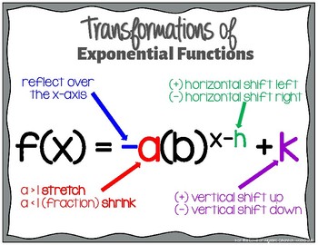
Vertical scaling: multiplying by a constant changes the initial value

Vertical translation: adding a constant shifts the graph up or down

Horizontal translation: replacing \( \mathrm{x} \) with \( \mathrm{x-h} \) shifts the graph left or right

Horizontal dilation: replacing \( \mathrm{x} \) with \( \mathrm{cx} \) stretches or compresses the graph

By combining these transformations, an exponential function can be tailored to accurately model real-world behavior.

Example

A population grows exponentially with a base growth factor of 1.1 and starts at 500 individuals. Due to a baseline adjustment, 50 individuals are added to the model.

Construct an exponential model.

▶️ Answer/Explanation

The initial exponential model is

\( \mathrm{ \displaystyle f(x) = 500(1.1)^x } \)

Adding a vertical translation of 50 gives

\( \mathrm{ \displaystyle g(x) = 500(1.1)^x + 50 } \)

Conclusion

The model reflects exponential growth with a vertical shift.

Example

A bacteria culture initially has 200 cells and doubles every 3 hours.

Construct an exponential model.

▶️ Answer/Explanation

Doubling corresponds to a base of 2.

Since the doubling occurs every 3 hours, apply a horizontal dilation:

\( \mathrm{ \displaystyle f(x) = 200 \cdot 2^{\tfrac{x}{3}} } \)

Conclusion

The model accounts for both the initial value and the growth rate over time.

Exponential Regression Using Technology

When a data set shows approximately proportional change over equal-length input-value intervals, an exponential function model can be constructed using technology through exponential regression.

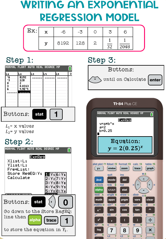
Exponential regression uses computational tools to find the exponential function of the form

\( \mathrm{ \displaystyle f(x) = ab^x } \)

that best fits the given data.

The technology determines values of \( \mathrm{a} \) (the initial value) and \( \mathrm{b} \) (the growth or decay factor) by minimizing the overall error between the model and the data.

This approach is especially useful when data does not follow an exact exponential pattern due to measurement error or real-world variability.

Key Idea

• Exponential regression finds a best-fit exponential model

• Technology is used when exact ratios are not constant

Example

The following data shows the population of a bacteria culture over time:

Time (hours): \( \mathrm{0,\;1,\;2,\;3} \)

Population: \( \mathrm{120,\;165,\;230,\;315} \)

Use exponential regression to model the data.

▶️ Answer/Explanation

Using exponential regression on a calculator or software gives a model close to

\( \mathrm{ \displaystyle f(x) \approx 120(1.38)^x } \)

Interpretation

The initial population is approximately 120, and the population increases by about 38% each hour.

Example

A data set records the value of a phone over several years:

Year: \( \mathrm{0,\;1,\;2,\;3} \)

Value (\$): \( \mathrm{800,\;680,\;575,\;490} \)

Use exponential regression to model the data.

▶️ Answer/Explanation

Using exponential regression gives a model close to

\( \mathrm{ \displaystyle f(x) \approx 800(0.85)^x } \)

Interpretation

The phone loses about 15% of its value each year.

The Natural Base \( \mathrm{e} \) in Exponential Models

The number \( \mathrm{e} \), called the natural base, is an irrational constant approximately equal to

\( \mathrm{ \displaystyle e \approx 2.718 } \)

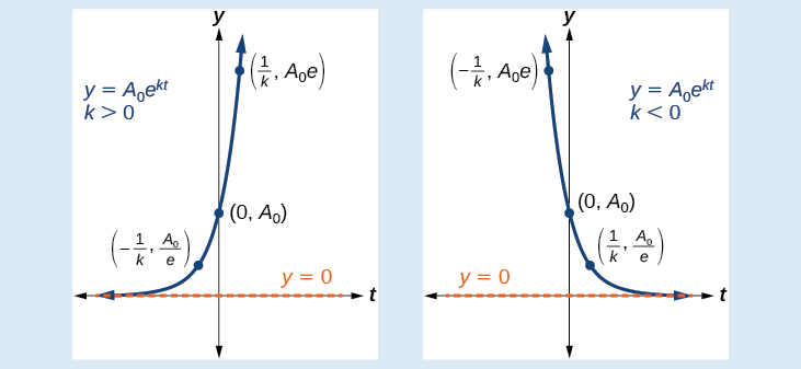
Exponential functions that use this base are written in the form

\( \mathrm{ \displaystyle f(x) = ae^x } \)

or, more generally,

\( \mathrm{ \displaystyle f(x) = ae^{kx} } \)

where \( \mathrm{a} \) is the initial value and \( \mathrm{k} \) is a constant growth or decay rate.

The base \( \mathrm{e} \) is commonly used in contextual scenarios involving continuous growth or decay, such as population growth, continuously compounded interest, radioactive decay, and cooling or heating processes.

Using base \( \mathrm{e} \) simplifies mathematical analysis and accurately models situations where change occurs continuously rather than in discrete steps.

Example

A population grows continuously at a rate of 5% per year and starts with 1,000 individuals.

Write an exponential model using base \( \mathrm{e} \).

▶️ Answer/Explanation

The initial value is \( \mathrm{a = 1000} \).

A continuous growth rate of 5% corresponds to \( \mathrm{k = 0.05} \).

\( \mathrm{ \displaystyle f(x) = 1000e^{0.05x} } \)

Conclusion

The model represents continuous exponential growth using the natural base.

Example

A substance decays continuously so that 30% of it is lost each year. The initial amount is 500 grams.

Write an exponential model using base \( \mathrm{e} \).

▶️ Answer/Explanation

A continuous decay rate of 30% corresponds to \( \mathrm{k = -0.30} \).

The initial value is \( \mathrm{a = 500} \).

\( \mathrm{ \displaystyle f(x) = 500e^{-0.30x} } \)

Conclusion

The model describes continuous exponential decay using the natural base.

Interpreting the Base of an Exponential Model

For an exponential model in general form

\( \mathrm{ \displaystyle f(x) = ab^x } \)

the base \( \mathrm{b} \) represents the growth factor or decay factor for successive unit changes in the input values.

Specifically, when the input increases by 1 unit, the output is multiplied by \( \mathrm{b} \):

\( \mathrm{ \displaystyle f(x+1) = b \cdot f(x) } \)

The base \( \mathrm{b} \) is directly related to percent change in contextual situations.

If the quantity grows by \( \mathrm{r\%} \) each unit of input, then

\( \mathrm{ \displaystyle b = 1 + \dfrac{r}{100} } \)

If the quantity decreases by \( \mathrm{r\%} \) each unit of input, then

\( \mathrm{ \displaystyle b = 1 – \dfrac{r}{100} } \)

Thus, the base \( \mathrm{b} \) encodes the rate of change of the exponential model in a meaningful real-world way.

Example

A population increases by 12% each year.

Write the exponential growth factor.

▶️ Answer/Explanation

A 12% increase corresponds to \( \mathrm{r = 12} \).

So the growth factor is

\( \mathrm{ \displaystyle b = 1 + \dfrac{12}{100} = 1.12 } \)

Conclusion

Each year, the population is multiplied by 1.12.

Example

The value of a machine decreases by 8% each year.

Identify the decay factor.

▶️ Answer/Explanation

An 8% decrease corresponds to \( \mathrm{r = 8} \).

So the decay factor is

\( \mathrm{ \displaystyle b = 1 – \dfrac{8}{100} = 0.92 } \)

Conclusion

Each year, the value is multiplied by 0.92.

Equivalent Forms of Exponential Functions

Equivalent forms of an exponential function can highlight different interpretations of the same growth process, depending on the context and the chosen unit of input.

Consider the exponential function

\( \mathrm{ \displaystyle f(d) = 2^d } \)

where \( \mathrm{d} \) represents the number of days.

In this form, the base \( \mathrm{2} \) shows that the quantity doubles every day.

Using exponent rules, the same function can be rewritten as

\( \mathrm{ \displaystyle f(d) = \left(2^7\right)^{\tfrac{d}{7}} } \)

This equivalent form expresses the growth in terms of weeks rather than days.

Here, the base \( \mathrm{2^7} \) indicates that the quantity increases by a factor of \( \mathrm{2^7} \) every 7 days (one week).

Although the algebraic forms look different, they represent the same function and the same growth behavior. The choice of form simply emphasizes different time scales or units in context.

Example

A quantity triples every day and is modeled by

\( \mathrm{ \displaystyle f(d) = 3^d } \)

Rewrite the function to show the growth factor per week.

▶️ Answer/Explanation

Use the exponent rule:

\( \mathrm{ \displaystyle 3^d = \left(3^7\right)^{\tfrac{d}{7}} } \)

Interpretation

The quantity increases by a factor of \( \mathrm{3^7} \) every 7 days.

Example

A population grows by a factor of 1.5 each day.

Write an equivalent exponential model that shows the growth per 10-day period.

▶️ Answer/Explanation

The daily model is

\( \mathrm{ \displaystyle f(d) = 1.5^d } \)

Rewrite using a 10-day interval:

\( \mathrm{ \displaystyle f(d) = \left(1.5^{10}\right)^{\tfrac{d}{10}} } \)

Interpretation

The population increases by a factor of \( \mathrm{1.5^{10}} \) every 10 days.

Using Exponential Models for Prediction

Exponential models can be used to predict values of the dependent variable by evaluating the model at specific input values.

A general exponential model has the form

\( \mathrm{ \displaystyle f(x) = ab^x } \)

Predictions made using an exponential model must respect the contextual constraints on the domain. These constraints determine which input values are meaningful.

For example:

• Time may be restricted to nonnegative values

• Inputs may be limited to whole numbers if the context involves discrete steps

• Predictions far outside the observed data range may be unreliable

When the domain is appropriately restricted, evaluating the exponential model provides reasonable predictions for future or past values.

Example

A population is modeled by the exponential function

\( \mathrm{ \displaystyle f(t) = 500(1.08)^t } \)

where \( \mathrm{t} \) represents time in years and \( \mathrm{t \ge 0} \).

Predict the population after 5 years.

▶️ Answer/Explanation

Substitute \( \mathrm{t = 5} \) into the model:

\( \mathrm{ \displaystyle f(5) = 500(1.08)^5 } \)

Evaluate:

\( \mathrm{ \displaystyle f(5) \approx 734 } \)

Conclusion

The predicted population after 5 years is approximately 734 individuals.

Example

The value of a machine is modeled by

\( \mathrm{ \displaystyle f(t) = 12000(0.9)^t } \)

where \( \mathrm{t} \) represents time in years and \( \mathrm{t} \) must be a whole number.

Predict the value after 3 years.

▶️ Answer/Explanation

Substitute \( \mathrm{t = 3} \) into the model:

\( \mathrm{ \displaystyle f(3) = 12000(0.9)^3 } \)

Evaluate:

\( \mathrm{ \displaystyle f(3) \approx 8748 } \)

Conclusion

The predicted value of the machine after 3 years is approximately \$8,748.

Scroll to Top