AP Precalculus -2.6 Competing Function Models- MCQ Exam Style Questions - Effective Fall 2023

AP Precalculus -2.6 Competing Function Models- MCQ Exam Style Questions – Effective Fall 2023

AP Precalculus -2.6 Competing Function Models- MCQ Exam Style Questions – AP Precalculus- per latest AP Precalculus Syllabus.

AP Precalculus – MCQ Exam Style Questions- All Topics

Question

A food vendor developed a new sandwich type for sale. The vendor made estimates about the sales of the new sandwich type over time. A linear regression was used to develop a model for the sales over time. The figure shows a graph of the residuals of the linear regression. Which of the following statements about the linear regression is true?

(A) The linear model is not appropriate, because there is a clear pattern in the graph of the residuals.
(B) The linear model is not appropriate, because the graph of the residuals has more points above 0 than below 0.
(C) The linear model is appropriate, because there is a clear pattern in the graph of the residuals.
(D) The linear model is appropriate, because the positive residual farthest from 0 and the negative residual farthest from 0 are about the same distance, although more points are above 0 than below 0.

▶️ Answer/Explanation

Detailed solution

If residuals show a clear pattern (curved shape, systematic deviation), the linear model is not appropriate.
From the description/figure (not shown here), residuals likely show a pattern.
✅ Answer: (A)

Question

The increasing function $ P $ gives the number of followers, in thousands, for a new musical group on a social media site. The table gives values of $ P(t) $ for selected values of $ t $, in months, since the musical group created their account on this social media site.

$ t $ (months)	0	1	2	3	4
$ P(t) $ (thousands)	20	30	45	67.5	101.25

If a model is constructed to represent these data, which of the following best applies to this situation?
(A) $ y = 10t + 20 $
(B) $ y = \frac{325}{16} t + 20 $
(C) $ y = 20\left(\frac{2}{3}\right)^t $
(D) $ y = 20\left(\frac{3}{2}\right)^t $

▶️ Answer/Explanation

Detailed solution

Observe the ratios of consecutive outputs:
$ 30/20 = 1.5 $, $ 45/30 = 1.5 $, $ 67.5/45 = 1.5 $, $ 101.25/67.5 = 1.5 $.
Constant ratio $ 1.5 = \frac{3}{2} $ indicates exponential growth: $ P(t) = a \cdot \left(\frac{3}{2}\right)^t $.
Using $ P(0) = 20 $ gives $ a = 20 $.
Thus $ P(t) = 20\left(\frac{3}{2}\right)^t $.
✅ Answer: (D)

Question

A regression model $S$ is constructed for a data set. The residuals from the regression are plotted and labeled. Based on the vertical axis of the residual plot (not shown), point $A$ is located at $1.3$ and point $B$ is located at $-2.5$. Which of the following statements is true about the model and the estimates produced by the model that correspond to $A$ and $B$?

(A) The model produces an overestimate at $A$ and an underestimate at $B$. Based on the absolute values of the residuals, there is a greater error in the model with $B$ than with $A$.
(B) The model produces an underestimate at $A$ and an overestimate at $B$. Based on the absolute values of the residuals, there is a greater error in the model with $B$ than with $A$.
(C) The model produces an overestimate at $A$ and an underestimate at $B$. Based on the absolute values of the residuals, there is a greater error in the model with $A$ than with $B$.
(D) The model produces an underestimate at $A$ and an overestimate at $B$. Based on the absolute values of the residuals, there is a greater error in the model with $A$ than with $B$.

▶️ Answer/Explanation

Detailed solution

1. Understand Residuals:
$\text{Residual} = \text{Actual} – \text{Predicted}$.

2. Analyze Point A (Residual = 1.3):
$1.3 > 0$, so $\text{Actual} > \text{Predicted}$. The model underestimated the value.

3. Analyze Point B (Residual = -2.5):
$-2.5 < 0$, so $\text{Actual} < \text{Predicted}$. The model overestimated the value.

4. Compare Errors:
The magnitude of the error is the absolute value of the residual.
Error at A: $|1.3| = 1.3$
Error at B: $|-2.5| = 2.5$
Since $2.5 > 1.3$, the error is greater with B.

✅ Answer: (B)

Question

(A) $ y = 10t + 20 $
(B) $ y = \frac{325}{16}t + 20 $
(C) $ y = 20\left(\frac{2}{3}\right)^t $
(D) $ y = 20\left(\frac{3}{2}\right)^t $

▶️ Answer/Explanation

Detailed solution

Check ratios:
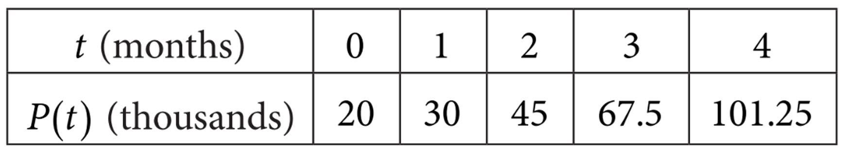
$ P(1)/P(0) = 30/20 = 1.5 $
$ P(2)/P(1) = 45/30 = 1.5 $
$ P(3)/P(2) = 67.5/45 = 1.5 $
$ P(4)/P(3) = 101.25/67.5 = 1.5 $
Constant ratio ⇒ exponential growth with base $ b = 1.5 = \frac{3}{2} $.
Initial value $ P(0) = 20 $ ⇒ $ a = 20 $.
Thus $ P(t) = 20 \left( \frac{3}{2} \right)^t $.
✅ Answer: (D)

Question

A relation between $y$ being test scores and $x$ being amount of time studying was transformed by plotting all points according to $(x, \log y)$. A linear regression was plotted using the transformed data set and the residual plot is below. What should be concluded from this data?

a. An exponential regression is not appropriate for this data set.
b. A logarithmic regression is not appropriate for this data set.
c. An exponential regression is appropriate for this data set.
d. A logarithmic regression is appropriate for this data set.

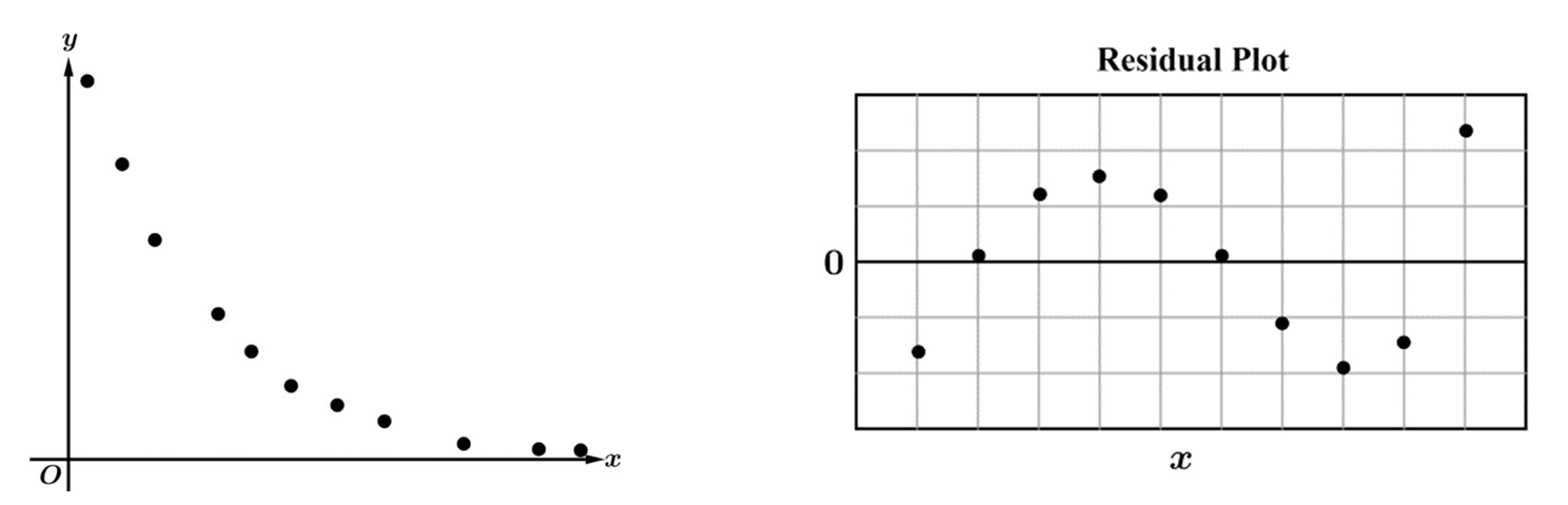
▶️ Answer/Explanation

Detailed solution

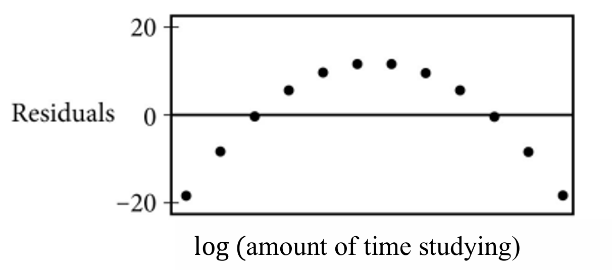
The transformation used is $(x, \log y)$, which is the standard method to linearize an exponential model.
A residual plot shows the difference between the observed values and the values predicted by the regression line.
The provided residual plot shows a clear distinct curved pattern (a parabolic shape).
In statistics, a patterned residual plot indicates that the chosen model is not a good fit for the data.
Since the linear model was applied to $(x, \log y)$, this “bad fit” refers to the underlying exponential relationship.
Therefore, an exponential regression is not appropriate for this specific data set.

Correct Option: a

Question

A linear regression was used to create a model for a set of data. The figure shows a graph of the residuals of the linear regression. Which of the following statements about the linear regression is true?

(A) A linear regression model is appropriate, because the residuals show a clear pattern.
(B) A linear regression model is appropriate, but a quadratic regression may be a better model.
(C) A linear regression model is not appropriate, because the residuals do not show a linear pattern.
(D) A linear regression model is not appropriate, because the residuals show a clear pattern.

▶️ Answer/Explanation

Detailed solution

The correct option is (D).
A residual plot should show a random scatter of points if a linear model is appropriate.
In this graph, the residuals exhibit a distinct $U$-shaped or curved pattern.
The presence of a non-random pattern indicates that the linear model fails to capture the underlying trend.
Therefore, the linear regression is not appropriate for this specific dataset.
This pattern suggests that a nonlinear model, such as a quadratic one, would be a better fit.
Option (D) correctly identifies that the pattern itself is the reason for the model’s inappropriateness.

Question

A regression model was created for the data in the graph above (left). The residual plot for the model is given above (right). Which of the following statements about the regression model is best?

(A) A quadratic regression model was used and the model is appropriate.

(B) A quadratic regression model was used and the model is not appropriate.

(D) An exponential regression model was used and the model is not appropriate.

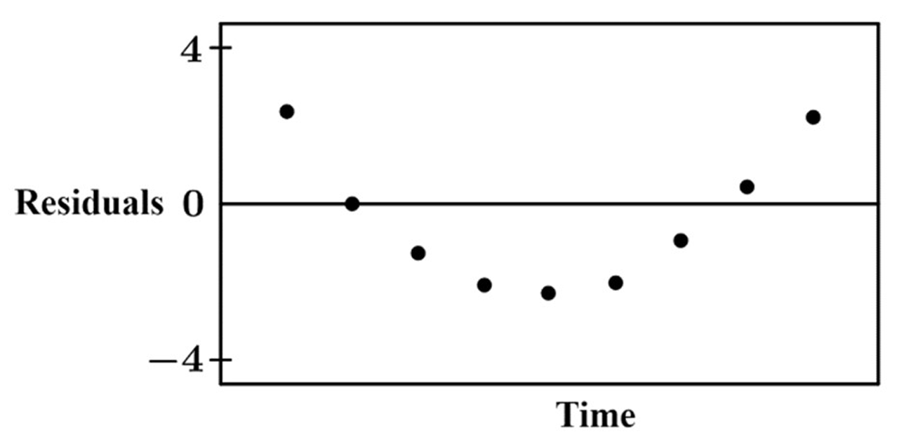
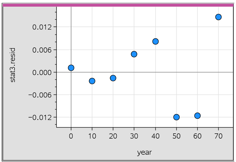
▶️ Answer/Explanation

Detailed solution

The correct option is (B).
The residual plot shows a distinct curved, non-random pattern (a “U” or “inverted U” shape).
A curved pattern in a residual plot indicates that the model used is not appropriate for the data.
The original scatterplot shows a curved relationship that could be modeled by a quadratic function $y = ax^2 + bx + c$.
However, since the residuals are not randomly scattered around the $y = 0$ line, a quadratic fit fails to capture the full trend.
For a model to be appropriate, the residuals should be randomly distributed with no discernible pattern.
Therefore, the quadratic model was used, but the resulting pattern in the residuals proves it is not the best fit.

Question

Mr. Passwater believed a set of data displayed exponential growth. He used the set of data to create an exponential regression model. The residual plot for his model is shown below. Based on the residual plot above, which of the following conclusions is correct?

(A) The residual plot has no apparent pattern, so the exponential model was appropriate.
(B) The residual plot has no apparent pattern, so the exponential model was not appropriate.
(C) The residual plot displays a pattern, so the exponential model was appropriate.
(D) The residual plot displays a pattern, so the exponential model was not appropriate.

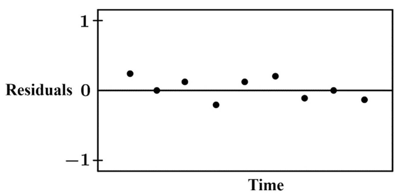
▶️ Answer/Explanation

Detailed solution

The correct option is (A).
A residual is calculated as $\text{observed value} – \text{predicted value}$.
The provided residual plot shows points randomly scattered above and below the line $y = 0$.
There is no curved, U-shaped, or systematic pattern visible in the residuals.
A random distribution of residuals indicates that the chosen model fits the data well.
Since there is no apparent pattern, the exponential regression model is considered appropriate.
Therefore, the data confirms Mr. Passwater’s belief regarding the exponential growth.

Question

A set of data was used to create a linear, a quadratic, and an exponential regression model. The residual plots for the three models are shown above. Based on the three residual plots, which of the following could be an appropriate model for the data?

(A) $y = 3x + 1$

(B) $y = x^2 – 3x + 1$

(D) $y = 1 + \log_3 x$

▶️ Answer/Explanation

Detailed solution

Correct Answer: (C) $y = 4(3)^x$

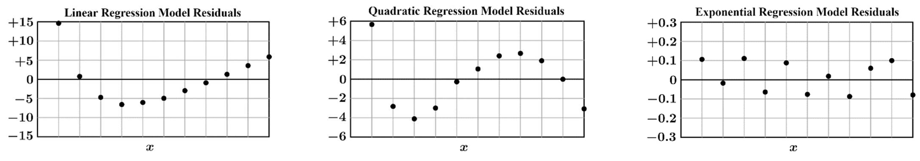
An appropriate regression model is indicated by a residual plot with no clear pattern and points randomly dispersed around the horizontal axis.
The Linear Residual Plot shows a distinct U-shaped pattern, suggesting a linear model is inappropriate.
The Quadratic Residual Plot also shows a clear curved pattern, indicating the quadratic model does not fit well.
The Exponential Residual Plot shows a random distribution of points above and below the $x$-axis.
Since the exponential residual plot is the most random, an exponential model is the best fit.
Option (C) represents an exponential function, $y = 4(3)^x$, making it the appropriate choice.

Question

A set of data and the linear regression model constructed for the data set are shown in the figure, along with data point $P$. Which of the following is the best estimate of the residual for data point $P$?

(A) $-0.5$
(B) $0.5$
(C) $1.5$
(D) $3$

▶️ Answer/Explanation

Detailed solution

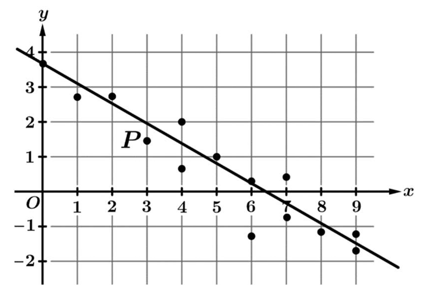
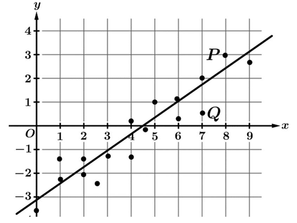
The residual is defined as the difference between the observed $y$-value and the predicted $\hat{y}$-value: $\text{Residual} = y – \hat{y}$.
Locate data point $P$ on the graph at the $x$-coordinate of $3$.
The actual $y$-value for point $P$ is $1.5$.
The predicted value $\hat{y}$ on the regression line at $x = 3$ is $2$.
Calculate the residual: $1.5 – 2 = -0.5$.
Therefore, the best estimate of the residual is $-0.5$.
The correct option is (A).

Question

An exponential regression model $S$ is constructed for a data set. The model $S$ is given by $S(x) = 3(2)^x$. The coordinates of a point $P$ from the data set are $(-1, 1)$. Which of the following statements is true about the residual of point $P$?

(A) The residual of point $P$ is a negative value because the model produces an overestimate at point $P$.
(B) The residual of point $P$ is a negative value because the model produces an underestimate at point $P$.
(C) The residual of point $P$ is a positive value because the model produces an overestimate at point $P$.
(D) The residual of point $P$ is a positive value because the model produces an underestimate at point $P$.

▶️ Answer/Explanation

Detailed solution

The correct option is (A).
Calculate the predicted value: $S(-1) = 3(2)^{-1} = 3(0.5) = 1.5$.
The actual $y$-coordinate of point $P$ is $1$.
The residual is calculated as $\text{Actual} – \text{Predicted} = 1 – 1.5 = -0.5$.
Since the residual is negative, the predicted value is greater than the actual value.
Therefore, the model produces an overestimate at point $P$.

Question

The figure shows a data set and its linear regression model in the $xy\text{-plane}$. The points $P$ and $Q$ are labeled. Which of the following statements is true about the model and the estimates produced by the model that correspond to $P$ and $Q$?

(A) The residuals for $P$ and $Q$ have the same sign. Based on the absolute value of the residuals, there is a greater error in the model with $P$ than with $Q$.

(B) The residuals for $P$ and $Q$ have the same sign. Based on the absolute value of the residuals, there is a greater error in the model with $Q$ than with $P$.

(C) The residuals for $P$ and $Q$ have opposite signs. Based on the absolute value of the residuals, there is a greater error in the model with $P$ than with $Q$.

(D) The residuals for $P$ and $Q$ have opposite signs. Based on the absolute value of the residuals, there is a greater error in the model with $Q$ than with $P$.

▶️ Answer/Explanation

Detailed solution

Point $P$ is above the regression line, meaning it has a positive residual.
Point $Q$ is below the regression line, meaning it has a negative residual.
Since one is positive and one is negative, the residuals have opposite signs.
The vertical distance from $Q$ to the line is visually larger than the distance from $P$ to the line.
The absolute value of a residual represents the magnitude of error for that point.
Therefore, there is a greater error in the model for point $Q$ than for point $P$.
This matches statement (D).

Question

The increasing function $P$ gives the number of followers, in thousands, for a new musical group on a social media site. The table gives values of $P(t)$ for selected values of $t$, in months, since the musical group created their account on this social media site. If a model is constructed to represent these data, which of the following best applies to this situation?

(A) $ y = 10t + 20 $

(B) $ y = \frac{325}{16}t + 20 $

(D) $ y = 20 \left(\frac{3}{2}\right)^t $

▶️ Answer/Explanation

Detailed solution

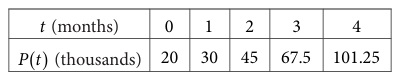
The differences between consecutive $P(t)$ values ($30-20=10$, $45-30=15$) are not constant, so the model is not linear (eliminates A and B).
Calculate the ratio of consecutive terms: $\frac{30}{20} = 1.5$ and $\frac{45}{30} = 1.5$.
Since the ratio is constant at $1.5$ or $\frac{3}{2}$, the data represents an exponential growth model.
An exponential function has the form $y = a(b)^t$, where $a$ is the initial value and $b$ is the growth factor.
From the table, at $t=0$, the value is $20$, so the initial value $a = 20$.
The growth factor $b$ is the constant ratio $\frac{3}{2}$.
Therefore, the function is $y = 20 \left(\frac{3}{2}\right)^t$, which corresponds to option (D).

Question

A table of values is given for a data set that can be modeled with $y$ as a function of $x$. Two function models, linear and exponential, are constructed using regressions. Residual plots for the two regressions are shown. Which of the following statements is true?

(A) A linear model is more appropriate for these data, and Residual Plot 1 corresponds to the linear regression.
(B) A linear model is more appropriate for these data, and Residual Plot 2 corresponds to the linear regression.
(C) An exponential model is more appropriate for these data, and Residual Plot 1 corresponds to the exponential regression.
(D) An exponential model is more appropriate for these data, and Residual Plot 2 corresponds to the exponential regression.

▶️ Answer/Explanation

Detailed solution

The correct answer is (D).
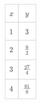
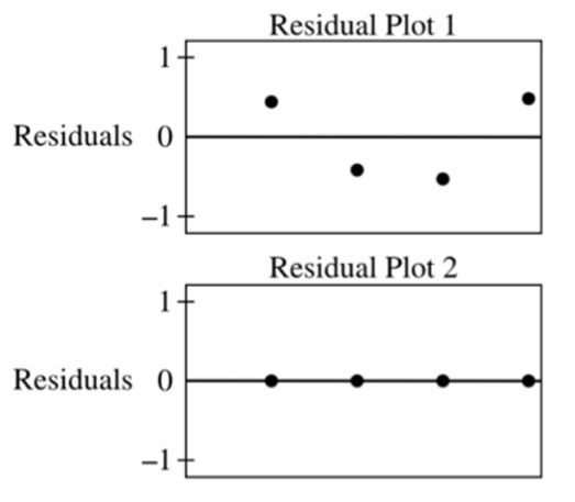
Analysis of the $y$-values shows a constant ratio: $\frac{9/2}{3} = \frac{27/4}{9/2} = \frac{81/8}{27/4} = 1.5$.
A constant ratio indicates that the data is perfectly exponential.
Residual Plot 2 shows all residuals are exactly $0$, meaning the model fits the data perfectly.
Therefore, the exponential model is the most appropriate for this data set.
Residual Plot 2 corresponds to this perfect exponential fit.
Residual Plot 1 shows a pattern, which usually indicates an inappropriate model (likely the linear one).

Question (Calc allowed)

Two function models $k$ and $m$ are constructed to represent the sales of a product at a group of grocery stores. Both $k(t)$ and $m(t)$ represent the sales of the product, in thousands of units, after $t$ weeks for $t \geq 2$. If $k(t) = 14 – 2.885 \ln t$ and $m(t) = -t + 14$, what is the first time $t$ that sales predicted by the logarithmic model will be $0.1$ thousand units more than sales predicted by the linear model?

(A) $t = 6.318$

(B) $t = 4.324$

(D) $t = 2.289$

▶️ Answer/Explanation

Detailed solution

Set up the equation where the logarithmic model exceeds the linear model by $0.1$: $k(t) = m(t) + 0.1$.
Substitute the given functions: $14 – 2.885 \ln t = (-t + 14) + 0.1$.
Simplify the equation to: $-2.885 \ln t = -t + 0.1$.
Rearrange to form the function: $f(t) = t – 2.885 \ln t – 0.1 = 0$.
Use a graphing calculator to find the intersection of $y = 14 – 2.885 \ln t$ and $y = -t + 14.1$.
The first intersection point for $t \geq 2$ occurs at $t \approx 2.289$.
Thus, the correct option is (D).

Question

The table shows values for a function $f$ at selected values of $x$. Which of the following claim and explanation statements best fits these data?

(A) $f$ is best modeled by an exponential function, because the input values change proportionately as output values increase in equal-length intervals.
(B) $f$ is best modeled by an exponential function, because the output values change proportionately as input values increase in equal-length intervals.
(C) $f$ is best modeled by a logarithmic function, because the input values change proportionately as output values increase in equal-length intervals.
(D) $f$ is best modeled by a logarithmic function, because the output values change proportionately as input values increase in equal-length intervals.

▶️ Answer/Explanation

Detailed solution

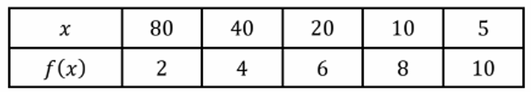
The correct option is (C).
As the output values $f(x)$ increase by a constant addition of $2$ ($2, 4, 6, 8, 10$),
the corresponding input values $x$ change by a constant factor of $1/2$ ($80, 40, 20, 10, 5$).
This relationship defines a logarithmic function, where inputs change geometrically while outputs change arithmetically.
In an exponential function, the roles are reversed: inputs change arithmetically and outputs change geometrically.
Therefore, $f$ is logarithmic because input values change proportionately as output values increase in equal-length intervals.
The specific model for this data is $f(x) = \log_{1/\sqrt{2}}(x/80) + 2$.

Question

In the $xy$-plane, the graphs of the linear function $L$ and the exponential function $E$ both pass through the points $(0,2)$ and $(1,6)$. The function $f$ is given by $f(x) = L(x) – E(x)$. What is the maximum value of $f$?

(A) $0.007$
(B) $0.172$
(C) $0.540$
(D) $1.002$

▶️ Answer/Explanation

Detailed solution

Find $L(x)$: Slope $m = \frac{6-2}{1-0} = 4$, so $L(x) = 4x + 2$.
Find $E(x)$: Form $y = ab^x$. At $x=0$, $a=2$; at $x=1$, $2b=6 \implies b=3$. So $E(x) = 2(3^x)$.
Define $f(x) = 4x + 2 – 2(3^x)$.
To find the maximum, set $f'(x) = 4 – 2(3^x)\ln(3) = 0$.
Solve for $x$: $3^x = \frac{2}{\ln(3)} \implies x = \frac{\ln(2/\ln(3))}{\ln(3)} \approx 0.544$.
Calculate $f(0.544) = 4(0.544) + 2 – 2(3^{0.544}) \approx 4.176 – 4.004 = 0.172$.
The correct option is (B).

Question

Over the years $1950 – 2020$, the total world population has been increasing. An exponential regression was used to develop a model for the population. The figure shows a graph of the residuals of the exponential regression. Which of the following statements about the exponential regression is true?

(A) The residual plot has no apparent pattern, so the exponential model was appropriate.

(B) The residual plot has no apparent pattern, so the exponential model was not appropriate.

(D) The residual plot displays a pattern, so the exponential model was not appropriate.

▶️ Answer/Explanation

Detailed solution

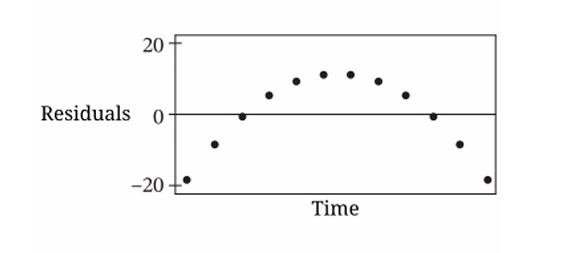
The correct option is (D).
The residual plot clearly shows a distinct $U$-shaped curve rather than a random scatter.
A visible pattern in a residual plot indicates that the chosen model (exponential) does not capture the underlying trend.
In statistics, a model is considered “appropriate” only if its residuals are randomly distributed around the horizontal axis.
Since a clear non-linear pattern exists, the exponential regression is an inappropriate fit for this specific data set.
Therefore, the presence of a pattern confirms the model’s inadequacy.

Question

An increasing, continuous function $ g(x) $ has outputs of some values of $ x $ shown above. $ f(x) $ is a function shown to the right as the graph.

(A) i. Estimate the value of $ g(f^{-1}(1)) $ for all values if it is defined.

ii. If $ h(x) = \frac{g(x)}{f(x)} $, then define any discontinuities, their type, and their location when $ x > 0 $.

(B) Suppose $ j(x) = \frac{1}{4.99 – \ln(x)} \cdot e^{2 \sin (\sqrt{x})} $ could be used to model $ f(x) $.

i. Determine the end behavior of $ j $ when it increases without bound. Express your answer with the mathematical definition of a limit if it exists. If it does not exist, explain why.

ii. Determine the vertical asymptote of $ j $ when it approaches $ 0 $ from the right. Express your answer with the mathematical definition of a limit if it exists. If it does not, explain why.

(C) Determine if $ g(x) $, using the values in the table, can be best modeled with a linear, quadratic, exponential, or logarithmic function. Explain your answer based on the relationship between the change in the output values of $ g $ and the change in the input values of $ g $.

Most-appropriate topic codes (CED):

• TOPIC 2.8: Inverses of Exponential Functions — part (A)i
• TOPIC 1.10: Rational Functions and Holes — part (A)ii
• TOPIC 1.7: Rational Functions and End Behavior — part (B)i
• TOPIC 1.9: Rational Functions and Vertical Asymptotes — part (B)ii
• TOPIC 2.10: Logarithmic Function Context and Data Modeling — part (C)

▶️ Answer/Explanation

Detailed solution

(A)

i. The graph of $ f(x) $ shows that $ f(2) \approx 1 $, so $ f^{-1}(1) \approx 2 $. From the table, $ g(2) = 1 $. Thus, $ g(f^{-1}(1)) \approx 1 $.
Since $ f(x) $ is continuous and increasing, the inverse is defined for values in its range.
The estimate is a single value, $ 1 $, as the graph aligns precisely with the point. No other values exist due to the strictly increasing nature of $ f(x) $.

ii. The graph of $ f(x) $ crosses zero at $ x=1 $, so $ f(1)=0 $, and from the table, $ g(1)=0 $.
Thus, $ h(1) $ is undefined ($ 0/0 $ form).
The limit as $ x \to 1 $ of $ h(x) $ exists and equals $ 1 $, since both $ g(x) $ and $ f(x) $ resemble $ \log_2(x) $, making $ h(x)=1 $ elsewhere.
This indicates a removable discontinuity at $ x=1 $. No other discontinuities for $ x>0 $, as $ f(x) \neq 0 $ elsewhere in the domain.
The location is $ x=1 $, type: removable.

(B)

i. As $ x \to \infty $, $ \ln(x) \to \infty $, so $ 4.99 – \ln(x) \to -\infty $, and $ \frac{1}{4.99 – \ln(x)} \to 0^- $.
The term $ e^{2 \sin(\sqrt{x})} $ oscillates between $ e^{-2} $ and $ e^{2} $, remaining bounded.
By the squeeze theorem, since the amplitude approaches $ 0 $, $ \lim_{x \to \infty} j(x) = 0 $.
The end behavior is that $ j(x) $ approaches $ 0 $. The limit exists.

ii. As $ x \to 0^+ $, $ \ln(x) \to -\infty $, so $ 4.99 – \ln(x) \to +\infty $, and $ \frac{1}{4.99 – \ln(x)} \to 0^+ $.
Also, $ \sqrt{x} \to 0^+ $, $ \sin(\sqrt{x}) \to 0^+ $, so $ e^{2 \sin(\sqrt{x})} \to e^0 = 1 $.
Thus, $ j(x) \to 0 \cdot 1 = 0 $.
The limit is $ \lim_{x \to 0^+} j(x) = 0 $.
No vertical asymptote at $ x=0 $, as the function approaches a finite value, not $ \pm \infty $.

(C)

The table shows $ g(x) $ values: at $ x=0.5, 1, 2, 4, 7, 8 $, $ g(x)=-1, 0, 1, 2, 2.807, 3 $.
When $ x $ doubles ($ 0.5 $ to $ 1 $, $ 1 $ to $ 2 $, $ 2 $ to $ 4 $, $ 4 $ to $ 8 $), $ \Delta g = +1 $ consistently.
This pattern matches logarithmic functions, where outputs increase by a constant for multiplicative input changes.
Linear would require constant $ \Delta g $ for constant $ \Delta x $, but $ \Delta x $ varies while $ \Delta g =1 $ for doublings.
Quadratic would show constant second differences, but here first differences are not constant.
Exponential would show constant ratios in outputs for additive input changes, which does not fit.
Thus, best modeled by a logarithmic function like $ g(x) = \log_2(x) $.

Question

A student won $500$ in an art contest. At first, the student kept the money in a desk. After $10$ months, the student deposited the money in a savings account that earned interest. Six months after depositing the money ($t = 6$), the amount in the account is $508.67$. Twelve months after depositing the money ($t = 12$), the amount in the account is $517.50$.

The amount of money the student has can be modeled by the piecewise function $M$ given by: $$M(t) = \begin{cases} 500 & \text{for } -10 \le t < 0 \\ ab^{(t/12)} & \text{for } t \ge 0 \end{cases}$$ where $M(t)$ is the amount, in dollars, at time $t$ months since the $500$ was deposited into the savings account. A negative value for $t$ represents the number of months before the student deposited the $500$ into the savings account.

Part A

(i) Use the given data to write two equations that can be used to find the values for constants $a$ and $b$ in the expression for $M(t)$.

(ii) Find the values for $a$ and $b$ as decimal approximations.

Part B

(i) Use the given data to find the average rate of change of the amount of money the student has, in dollars per month, from $t = -2$ to $t = 12$ months. Express your answer as a decimal approximation. Show the computations that lead to your answer.

(ii) Use $M(12)$ and the average rate of change found in (i) to estimate the amount of money, in dollars, the student has when $t = 20$ months. Show the work that leads to your answer.

(iii) Let $A(t)$ be the estimate of the amount of money, in dollars, the student has at time $t$ months using the average rate of change found in (i). If $A(t)$ is used to estimate values for $M(t)$ for $t > 12$, the error in the estimates will increase as $t$ increases. Explain why this is true.

Part C

The student plans to close the account when the amount of money in the account reaches $565$. Explain how this information can be used to determine the domain limitations for the model $M$.

▶️ Answer/Explanation

Detailed solution

Part A

(i)
Using the data $M(6) = 508.67$ and $M(12) = 517.50$:
$ab^{(6/12)} = 508.67$ (or $ab^{0.5} = 508.67$)
$ab^{(12/12)} = 517.50$ (or $ab = 517.50$)

(ii)
Divide the second equation by the first: $\frac{ab}{ab^{0.5}} = \frac{517.50}{508.67}$
$b^{0.5} \approx 1.017359…$
$b \approx (1.017359…)^2 \approx 1.035019…$
Using $ab = 517.50 \implies a = \frac{517.50}{1.035019…} \approx 500$
Final values: $a \approx 500.00$ and $b \approx 1.035$

Part B

(i)
$t = -2$ falls in the interval $-10 \le t < 0$, so $M(-2) = 500$.
$t = 12$ is given as $M(12) = 517.50$.
Average Rate of Change $= \frac{M(12) – M(-2)}{12 – (-2)}$
$= \frac{517.50 – 500}{12 + 2}$
$= \frac{17.50}{14} = 1.25$ dollars per month.

(ii)
The linear estimate $A(t)$ uses the point $(12, 517.50)$ and slope $1.25$.
$A(20) = M(12) + 1.25(20 – 12)$
$A(20) = 517.50 + 1.25(8)$
$A(20) = 517.50 + 10 = 527.50$ dollars.

(iii)
The model $M(t)$ for $t \ge 0$ is an exponential function ($b > 1$), which is concave up.
The estimate $A(t)$ is a linear function (a secant line).
Since $M(t)$ is increasing at an increasing rate (exponential growth), the linear model will fall further behind the actual values as $t$ increases.

Part C

The model is only valid as long as the account is open.
Setting $M(t) = 565$ allows us to solve for the maximum value of $t$.
$500(1.035)^{(t/12)} = 565$
This value of $t$ serves as the upper bound (maximum) for the domain of the model $M$.

Question

After Mr. Passwater missed a day of school, a rumor began to spread that he had won the Powerball lottery and moved to Japan. Initially, seven students knew about the rumor (they were the ones that started it!). After two hours ($t=2$), a total of 15 students had heard the rumor. After six hours ($t=6$), 67 students had heard the rumor.

The number of students that have heard the rumor can be modeled by the piecewise function $R$ given by: $$R(t) = \begin{cases} 7(a)^{t/2} & \text{for } 0 \le t < 6 \\ -213.29 + b \ln t & \text{for } t \ge 6 \end{cases}$$ where $R(t)$ is the number of students that have heard the rumor at time $t$ hours since the rumor first began.

(A) (i) Use the given data to write two equations that can be used to find the values for constants $a$ and $b$ in the expression for $R(t)$.
(ii) Find the values for $a$ and $b$ as decimal approximations.

(B) (i) Use the given data to find the average rate of change in the number of students that have heard the rumor, in students per hour, from $t=2$ to $t=6$ hours. Express your answer as a decimal approximation. Show the computations that lead to your answer.
(ii) Interpret the meaning of your answer from (i) in the context of the problem.
(iii) Consider the values that result from using the average rate of change found in (i) to estimate the number of students that have heard the rumor for times $t=p$ hours, where $0 < p < 6$. Are these estimates less than or greater than the number of students predicted by the model $R$ for times $t=p$ hours? Explain your reasoning using characteristics of the average rate of change and characteristics of the model $R$.

(C) The model $R$ is valid for $0 \le t \le 12$ hours. Explain how the range values of the function $R$ should be limited by the context of the problem.

▶️ Answer/Explanation

Detailed solution

Part (A)

(i) Writing the equations:
We are given the following data points:
• At $t=2$, $R(2) = 15$.
• At $t=6$, $R(6) = 67$.

For $t=2$, since $0 \le 2 < 6$, we use the first part of the piecewise function: $R(t) = 7(a)^{t/2}$.
$$15 = 7(a)^{2/2} \quad \Rightarrow \quad 15 = 7a^1$$
Equation 1: $15 = 7a$

For $t=6$, since $t \ge 6$, we use the second part of the piecewise function: $R(t) = -213.29 + b \ln t$.
Equation 2: $67 = -213.29 + b \ln(6)$

(ii) Finding the values for $a$ and $b$:
From Equation 1:
$$a = \frac{15}{7} \approx 2.1428$$
From Equation 2:
$$67 + 213.29 = b \ln(6)$$
$$280.29 = b \ln(6)$$
$$b = \frac{280.29}{\ln(6)} \approx \frac{280.29}{1.79176} \approx 156.4328$$
Answer: $a \approx 2.143$, $b \approx 156.433$

Part (B)

(i) Average Rate of Change:
The formula for the average rate of change from $t=2$ to $t=6$ is:
$$\text{Avg Rate} = \frac{R(6) – R(2)}{6 – 2}$$
Substituting the given values ($R(6)=67$ and $R(2)=15$):
$$\text{Avg Rate} = \frac{67 – 15}{4} = \frac{52}{4} = 13$$
Answer: 13 students per hour.

(ii) Interpretation:
On average, the number of students who have heard the rumor increases by 13 students per hour between the 2nd hour and the 6th hour.

(iii) Estimates vs. Model Prediction:
Answer: The estimates are greater than the number of students predicted by the model.
Reasoning:
• On the interval $0 < t < 6$, the function $R(t) = 7(a)^{t/2}$ is an exponential growth function with a base greater than 1.
• Exponential growth functions are concave up (the rate of change is increasing).
• The average rate of change corresponds to the slope of the secant line connecting the points at $t=2$ and $t=6$.
• For a concave up curve, the secant line lies above the curve on the interval between the two points. Therefore, linear estimates based on the average rate (secant line) will be greater than the actual function values.

Part (C)

Explanation:
The range values (outputs) of $R(t)$ represent the number of students. In the context of the problem, this range must be limited in two ways:
1. Population Cap: The number of students who heard the rumor cannot exceed the total student population of the school.
2. Discrete Values: You cannot have a fraction of a student, so strictly speaking, the context implies the range should consist of whole numbers (non-negative integers).

Question

The Chinese bamboo tree exhibits a unique growth pattern. Once a seed has been planted, the Chinese bamboo tree does not break through the ground for several years. However, once it breaks through the ground, the Chinese bamboo tree grows exponentially. In one particular experiment, a group of biologists recorded the height of a Chinese bamboo tree once it broke through the ground. After one week ($t = 1$), the Chinese bamboo tree measured 3 feet, and after five weeks ($t = 5$), the same tree measured 89 feet.

The height of the Chinese bamboo tree can be modeled by the function $H$ given by $H(t) = ab^x$, where $H(t)$ is the height of the tree, in feet, $t$ weeks after it first breaks ground.

(A) (i) Use the given data to write two equations that can be used to find the values for constants $a$ and $b$ in the expression for $H(t)$.

(ii) Find the values for $a$ and $b$.

(B) (i) Use the given data to find the average rate of change of the height of the Chinese bamboo tree, in feet per week, from $t = 1$ to $t = 5$ weeks. Express your answer as a decimal approximation. Show the computations that lead to your answer.

(ii) Interpret the meaning of your answer from (i) in the context of the problem.

(iii) Consider the average rates of change of $H$ from $t = 5$ to $t = p$ weeks, where $p > 5$. Are these average rates of change less than or greater than the average rate of change from $t = 1$ to $t = 5$ weeks found in (i)? Explain your reasoning.

(C) For which $t$-value, $t = 4$ weeks or $t = 11$ weeks, should the biologists have more confidence in when using the model $H$? Give a reason for your answer in the context of the problem.

▶️ Answer/Explanation

Detailed solution

(A)(i) Equations
Substituting the points $(1, 3)$ and $(5, 89)$ into $H(t) = ab^t$:
1. $3 = ab^1$ (or $3 = ab$)
2. $89 = ab^5$

(A)(ii) Values for a and b
Dividing equation 2 by equation 1: $\frac{ab^5}{ab} = \frac{89}{3} \implies b^4 = 29.67$.
Solving for $b$: $b = (29.67)^{0.25} \approx 2.33$.
Solving for $a$: $a = \frac{3}{2.33} \approx 1.29$.

(B)(i) Average Rate of Change
$\text{Rate} = \frac{H(5) – H(1)}{5 – 1} = \frac{89 – 3}{4} = \frac{86}{4} = 21.5$
Answer: 21.5 feet per week.

(B)(ii) Interpretation
The answer indicates that between the first and fifth weeks, the bamboo tree grew at an average speed of 21.5 feet per week.

(B)(iii) Comparison
Greater. The function represents exponential growth ($b > 1$), which is concave up. This means the rate of growth increases over time, so the rate after week 5 will be steeper than the rate before week 5.

(C) Confidence
$t = 4$ weeks.
The biologists should be more confident in $t=4$ because it is an interpolation (within the observed data range). $t=11$ is an extrapolation; biological growth cannot remain exponential indefinitely, so the model is likely inaccurate that far out.

AP Precalculus -2.6 Competing Function Models- MCQ Exam Style Questions - Effective Fall 2023