Linear Transformations
A linear transformation is a function that maps an input vector to an output vector.
Each component of the output vector is formed as the sum of constant multiples of the components of the input vector.
![]()
In two dimensions, a linear transformation can be written in matrix form as
\( \begin{pmatrix} x’ \\ y’ \end{pmatrix} = \begin{pmatrix} a & b \\ c & d \end{pmatrix} \begin{pmatrix} x \\ y \end{pmatrix} \)
This means
\( x’ = ax + by \)
\( y’ = cx + dy \)
Linear transformations are used to describe geometric operations such as rotations, reflections, stretches, and shears.
Example:
Let the linear transformation be defined by
\( T(\mathbf{v}) = \begin{pmatrix} 2 & 1 \\ -1 & 3 \end{pmatrix} \mathbf{v} \)
Find the image of the vector \( \mathbf{v} = \begin{pmatrix} 1 \\ 2 \end{pmatrix} \).
▶️ Answer/Explanation
Multiply the matrix by the vector:
\( T(\mathbf{v}) = \begin{pmatrix} 2(1) + 1(2) \\ -1(1) + 3(2) \end{pmatrix} = \begin{pmatrix} 4 \\ 5 \end{pmatrix} \)
Conclusion: The output vector is \( \begin{pmatrix} 4 \\ 5 \end{pmatrix} \).
Example:
Describe the transformation represented by the matrix
\( \begin{pmatrix} 3 & 0 \\ 0 & 1 \end{pmatrix} \)
▶️ Answer/Explanation
The output vector satisfies
\( x’ = 3x \), \( y’ = y \)
This stretches vectors horizontally by a factor of 3 while leaving vertical components unchanged.
Conclusion: The transformation is a horizontal stretch.
Matrix Representation of Linear Transformations in \( \mathbb{R}^2 \)
For a linear transformation \( L \) from \( \mathbb{R}^2 \) to \( \mathbb{R}^2 \), there exists a unique \( 2 \times 2 \) matrix \( A \) such that
\( L(\mathbf{v}) = A\mathbf{v} \)
for every vector \( \mathbf{v} \in \mathbb{R}^2 \).
This means that every linear transformation in \( \mathbb{R}^2 \) can be represented exactly by matrix multiplication.
Conversely, if \( A \) is any \( 2 \times 2 \) matrix, then the function defined by
\( L(\mathbf{v}) = A\mathbf{v} \)
is a linear transformation from \( \mathbb{R}^2 \) to \( \mathbb{R}^2 \).
This establishes a one-to-one correspondence between linear transformations in \( \mathbb{R}^2 \) and \( 2 \times 2 \) matrices.
Example:
Let the linear transformation \( L \) satisfy
\( L\!\left(\begin{pmatrix}1\\0\end{pmatrix}\right)= \begin{pmatrix}2\\1\end{pmatrix}, \quad L\!\left(\begin{pmatrix}0\\1\end{pmatrix}\right)= \begin{pmatrix}-1\\3\end{pmatrix} \)
Find the matrix \( A \) such that \( L(\mathbf{v}) = A\mathbf{v} \).
▶️ Answer/Explanation
The columns of \( A \) are the images of the standard basis vectors.
\( A = \begin{pmatrix} 2 & -1 \\ 1 & 3 \end{pmatrix} \)
Conclusion: This matrix uniquely represents the linear transformation \( L \).
Example:
Let
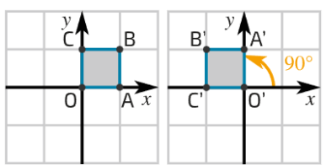
\( A = \begin{pmatrix} 0 & -1 \\ 1 & 0 \end{pmatrix} \)
Define \( L(\mathbf{v}) = A\mathbf{v} \). Describe the transformation.
▶️ Answer/Explanation
For \( \mathbf{v} = \begin{pmatrix}x\\y\end{pmatrix} \),
\( L(\mathbf{v}) = \begin{pmatrix}-y\\x\end{pmatrix} \)
This corresponds to a rotation of vectors by \( \dfrac{\pi}{2} \) radians counterclockwise about the origin.
Conclusion: Any \( 2 \times 2 \) matrix defines a linear transformation in \( \mathbb{R}^2 \).
Applying a Linear Transformation to Multiple Vectors
Let \( A \) be a \( 2 \times 2 \) matrix that represents a linear transformation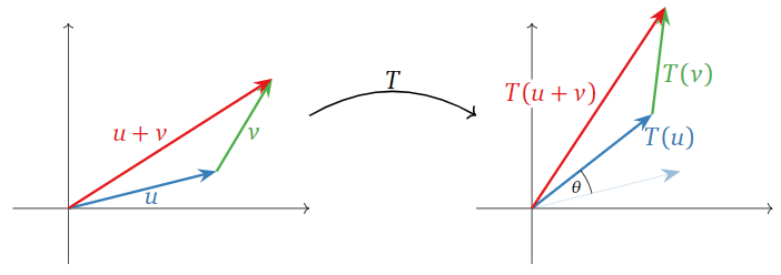
\( L(\mathbf{v}) = A\mathbf{v} \)
in \( \mathbb{R}^2 \).
If we have n input vectors in \( \mathbb{R}^2 \), they can be arranged as columns of a \( 2 \times n \) matrix
\( V = \begin{pmatrix} \mathbf{v}_1 & \mathbf{v}_2 & \dots & \mathbf{v}_n \end{pmatrix} \)
Multiplying the transformation matrix \( A \) by this matrix of input vectors produces a \( 2 \times n \) matrix of output vectors:
\( AV = \begin{pmatrix} A\mathbf{v}_1 & A\mathbf{v}_2 & \dots & A\mathbf{v}_n \end{pmatrix} \)
Each column of the resulting matrix is the image of the corresponding input vector under the linear transformation.
This method allows multiple vectors to be transformed simultaneously using a single matrix multiplication.
Example:
Let
\( A = \begin{pmatrix} 2 & 0 \\ 1 & 1 \end{pmatrix} \)
and let the input vectors be
\( V = \begin{pmatrix} 1 & 0 & -1 \\ 2 & 1 & 3 \end{pmatrix} \)
Find the matrix of output vectors.
▶️ Answer/Explanation
Multiply \( A \) by \( V \):
\( AV = \begin{pmatrix} 2 & 0 \\ 1 & 1 \end{pmatrix} \begin{pmatrix} 1 & 0 & -1 \\ 2 & 1 & 3 \end{pmatrix} = \begin{pmatrix} 2 & 0 & -2 \\ 3 & 1 & 2 \end{pmatrix} \)
Conclusion: Each column represents the transformed version of the corresponding input vector.
Example:
Explain why the product \( AV \) applies the transformation to each vector individually.
▶️ Answer/Explanation
Matrix multiplication operates column by column.
Each column of \( V \) is multiplied by \( A \), producing \( A\mathbf{v}_1, A\mathbf{v}_2, \dots, A\mathbf{v}_n \).
Conclusion: A single matrix multiplication applies the linear transformation to all input vectors at once.