Home / AP® Exam / AP® PreCalculus / AP® Precalculus

AP Precalculus -4.13 Matrices as Functions- Study Notes - Effective Fall 2023

AP Precalculus -4.13 Matrices as Functions- Study Notes – Effective Fall 2023

AP Precalculus -4.13 Matrices as Functions- Study Notes – AP Precalculus- per latest AP Precalculus Syllabus.

LEARNING OBJECTIVE

Determine the association between a linear transformation and a matrix.
Determine the composition of two linear transformations.
Determine the inverse of a linear transformation.

Key Concepts: 

  • Matrix Associated with a Linear Transformation in R2
  • Using Unit Vectors to Determine a Linear Transformation Matrix
  • Rotation Matrix in R2
  • Determinant and Area Scaling in Linear Transformations
  • Composition of Linear Transformations
  • Matrices and the Composition of Linear Transformations
  • Inverse of a Linear Transformation

AP Precalculus -Concise Summary Notes- All Topics

Matrix Associated with a Linear Transformation in \( \mathbb{R}^2 \)

A linear transformation that maps a point \( (x, y) \) to

\( \langle a_{11}x + a_{12}y,\; a_{21}x + a_{22}y \rangle \)

can be written using matrix multiplication.

The transformation is associated with the \( 2 \times 2 \) matrix

\( A = \begin{pmatrix} a_{11} & a_{12} \\ a_{21} & a_{22} \end{pmatrix} \)

so that the transformation can be written as

\( L(\mathbf{v}) = A\mathbf{v} \)

where

\( \mathbf{v} = \begin{pmatrix} x \\ y \end{pmatrix} \)

Each row of the matrix determines how the input components \( x \) and \( y \) are combined to produce one component of the output vector.

This matrix form provides a compact and consistent way to represent linear transformations.

Example:

Write the matrix associated with the transformation

\( L(x,y) = \langle 3x – y,\; 2x + 4y \rangle \)

▶️ Answer/Explanation

Identify the coefficients of \( x \) and \( y \) in each component.

\( A = \begin{pmatrix} 3 & -1 \\ 2 & 4 \end{pmatrix} \)

Conclusion: This matrix represents the given linear transformation.

Example:

Use the matrix

\( A = \begin{pmatrix} 1 & 2 \\ -3 & 1 \end{pmatrix} \)

to find the image of the point \( (2, -1) \).

▶️ Answer/Explanation

Write the input as a column vector and multiply:

\( A \begin{pmatrix} 2 \\ -1 \end{pmatrix} = \begin{pmatrix} 1(2) + 2(-1) \\ -3(2) + 1(-1) \end{pmatrix} = \begin{pmatrix} 0 \\ -7 \end{pmatrix} \)

Conclusion: The image of \( (2, -1) \) is \( (0, -7) \).

Using Unit Vectors to Determine a Linear Transformation Matrix

In \( \mathbb{R}^2 \), the unit vectors are

\( \mathbf{e}_1 = \begin{pmatrix}1 \\ 0\end{pmatrix} \), \( \mathbf{e}_2 = \begin{pmatrix}0 \\ 1\end{pmatrix} \)

For a linear transformation \( L \), knowing how these unit vectors are mapped completely determines the associated matrix.

If

\( L(\mathbf{e}_1) = \begin{pmatrix} a \\ c \end{pmatrix}, \quad L(\mathbf{e}_2) = \begin{pmatrix} b \\ d \end{pmatrix} \)

then the matrix associated with \( L \) is

\( A = \begin{pmatrix} a & b \\ c & d \end{pmatrix} \)

The images of the unit vectors form the columns of the transformation matrix.

This approach works because every vector in \( \mathbb{R}^2 \) can be written as a linear combination of the unit vectors.

Example:

Suppose a linear transformation \( L \) satisfies

\( L\!\left(\begin{pmatrix}1\\0\end{pmatrix}\right)= \begin{pmatrix}3\\-1\end{pmatrix}, \quad L\!\left(\begin{pmatrix}0\\1\end{pmatrix}\right)= \begin{pmatrix}2\\4\end{pmatrix} \)

Find the matrix associated with \( L \).

▶️ Answer/Explanation

Place the images of the unit vectors as columns:

\( A = \begin{pmatrix} 3 & 2 \\ -1 & 4 \end{pmatrix} \)

Conclusion: This matrix uniquely represents the transformation \( L \).

Example:

Explain why knowing \( L(\mathbf{e}_1) \) and \( L(\mathbf{e}_2) \) is sufficient to determine \( L(\mathbf{v}) \) for any vector \( \mathbf{v} \).

▶️ Answer/Explanation

Any vector \( \mathbf{v} = \begin{pmatrix}x\\y\end{pmatrix} \) can be written as

\( \mathbf{v} = x\mathbf{e}_1 + y\mathbf{e}_2 \)

Using linearity,

\( L(\mathbf{v}) = xL(\mathbf{e}_1) + yL(\mathbf{e}_2) \)

Conclusion: The transformation is completely determined by its effect on the unit vectors.

Rotation Matrix in \( \mathbb{R}^2 \)

The matrix

\( \begin{pmatrix} \cos \theta & -\sin \theta \\ \sin \theta & \cos \theta \end{pmatrix} \)

is associated with a linear transformation that rotates every vector in \( \mathbb{R}^2 \) by an angle \( \theta \) counterclockwise about the origin.

If a vector \( \mathbf{v} = \begin{pmatrix} x \\ y \end{pmatrix} \), then applying the rotation matrix gives

\( \begin{pmatrix} \cos \theta & -\sin \theta \\ \sin \theta & \cos \theta \end{pmatrix} \begin{pmatrix} x \\ y \end{pmatrix} = \begin{pmatrix} x\cos \theta – y\sin \theta \\ x\sin \theta + y\cos \theta \end{pmatrix} \)

This transformation preserves both the length of vectors and the angles between vectors, changing only their direction.

Special cases include:

\( \theta = 0 \): identity transformation

\( \theta = \dfrac{\pi}{2} \): rotation by 90° counterclockwise

\( \theta = \pi \): rotation by 180°

Example:

Rotate the vector \( (1, 0) \) by an angle \( \theta = \dfrac{\pi}{2} \) counterclockwise.

▶️ Answer/Explanation

For \( \theta = \dfrac{\pi}{2} \),

\( \cos \dfrac{\pi}{2} = 0 \), \( \sin \dfrac{\pi}{2} = 1 \)

Apply the rotation matrix:

\( \begin{pmatrix} 0 & -1 \\ 1 & 0 \end{pmatrix} \begin{pmatrix} 1 \\ 0 \end{pmatrix} = \begin{pmatrix} 0 \\ 1 \end{pmatrix} \)

Conclusion: The vector \( (1,0) \) is rotated to \( (0,1) \).

Example:

Find the image of the vector \( (2, 1) \) under a rotation of \( \theta = \pi \).

▶️ Answer/Explanation

For \( \theta = \pi \),

\( \cos \pi = -1 \), \( \sin \pi = 0 \)

Apply the rotation matrix:

\( \begin{pmatrix} -1 & 0 \\ 0 & -1 \end{pmatrix} \begin{pmatrix} 2 \\ 1 \end{pmatrix} = \begin{pmatrix} -2 \\ -1 \end{pmatrix} \)

Conclusion: A rotation by \( \pi \) maps \( (2,1) \) to \( (-2,-1) \).

Determinant and Area Scaling in Linear Transformations

For a linear transformation in \( \mathbb{R}^2 \) represented by a \( 2 \times 2 \) matrix \( A \), the absolute value of the determinant of \( A \) describes how areas change under the transformation.

Specifically,

\( |\det(A)| \)

gives the magnitude of the dilation of regions in \( \mathbb{R}^2 \).

This means that if a region in the plane has area \( S \), then after applying the transformation, the area becomes

\( |\det(A)| \cdot S \)

  • If \( |\det(A)| > 1 \), areas are enlarged.
  • If \( 0 < |\det(A)| < 1 \), areas are reduced.
  • If \( |\det(A)| = 1 \), areas are preserved.
  • If \( \det(A) = 0 \), all regions collapse to zero area.

Example:

Consider the transformation represented by

\( A = \begin{pmatrix} 2 & 0 \\ 0 & 3 \end{pmatrix} \)

Find the area scaling factor.

▶️ Answer/Explanation

Compute the determinant:

\( \det(A) = (2)(3) – (0)(0) = 6 \)

The absolute value is 6.

Conclusion: All regions have their area multiplied by a factor of 6.

Example:

A transformation preserves area. What must be true about the determinant?

▶️ Answer/Explanation

If areas are preserved, the scaling factor is 1.

Therefore,

\( |\det(A)| = 1 \)

Conclusion: The determinant must have absolute value 1.

Composition of Linear Transformations

The composition of two linear transformations is itself a linear transformation.

If \( L_1 \) and \( L_2 \) are linear transformations from \( \mathbb{R}^2 \) to \( \mathbb{R}^2 \), then their composition is defined by

\( (L_2 \circ L_1)(\mathbf{v}) = L_2(L_1(\mathbf{v})) \)

Because both transformations satisfy linearity, their composition also preserves linearity.

If \( L_1(\mathbf{v}) = A\mathbf{v} \) and \( L_2(\mathbf{v}) = B\mathbf{v} \), then the composed transformation is

\( (L_2 \circ L_1)(\mathbf{v}) = B(A\mathbf{v}) = (BA)\mathbf{v} \)

Thus, the matrix associated with the composition is the matrix product \( BA \).

The order of multiplication matters, since matrix multiplication is not commutative.

Example:

Let

\( L_1(\mathbf{v}) = \begin{pmatrix} 2 & 0 \\ 0 & 1 \end{pmatrix} \mathbf{v}, \quad L_2(\mathbf{v}) = \begin{pmatrix} 0 & -1 \\ 1 & 0 \end{pmatrix} \mathbf{v} \)

Find the matrix for \( L_2 \circ L_1 \).

▶️ Answer/Explanation

Multiply the matrices in the correct order:

\( BA = \begin{pmatrix} 0 & -1 \\ 1 & 0 \end{pmatrix} \begin{pmatrix} 2 & 0 \\ 0 & 1 \end{pmatrix} = \begin{pmatrix} 0 & -1 \\ 2 & 0 \end{pmatrix} \)

Conclusion: The composition is a linear transformation represented by this matrix.

Example:

Explain why the composition of two linear transformations must map the zero vector to the zero vector.

▶️ Answer/Explanation

Since each linear transformation maps the zero vector to the zero vector,

\( L_1(\mathbf{0}) = \mathbf{0} \) and \( L_2(\mathbf{0}) = \mathbf{0} \)

Applying the composition gives

\( (L_2 \circ L_1)(\mathbf{0}) = L_2(L_1(\mathbf{0})) = L_2(\mathbf{0}) = \mathbf{0} \)

Conclusion: The composition satisfies a key property of linear transformations.

Matrices and the Composition of Linear Transformations

When two linear transformations are composed, the resulting transformation can be represented by matrix multiplication.

Suppose

\( L_1(\mathbf{v}) = A\mathbf{v} \)

\( L_2(\mathbf{v}) = B\mathbf{v} \)

where \( A \) and \( B \) are \( 2 \times 2 \) matrices.

The composition of these transformations is

\( (L_2 \circ L_1)(\mathbf{v}) = L_2(L_1(\mathbf{v})) \)

Substituting the matrix forms gives

\( (L_2 \circ L_1)(\mathbf{v}) = B(A\mathbf{v}) = (BA)\mathbf{v} \)

Therefore, the matrix associated with the composition is the product of the matrices, taken in the correct order.

Important: The order of multiplication matters. In general,

\( BA \ne AB \)

The matrix closest to the vector corresponds to the transformation applied first.

Example:

Let

\( A = \begin{pmatrix} 1 & 2 \\ 0 & 1 \end{pmatrix}, \quad B = \begin{pmatrix} 0 & -1 \\ 1 & 0 \end{pmatrix} \)

Find the matrix associated with \( L_2 \circ L_1 \).

▶️ Answer/Explanation

Multiply the matrices in the correct order:

\( BA = \begin{pmatrix} 0 & -1 \\ 1 & 0 \end{pmatrix} \begin{pmatrix} 1 & 2 \\ 0 & 1 \end{pmatrix} = \begin{pmatrix} 0 & -1 \\ 1 & 2 \end{pmatrix} \)

Conclusion: The composition is represented by the matrix \( BA \).

Example:

Explain why reversing the order of multiplication represents a different transformation.

▶️ Answer/Explanation

Matrix multiplication is not commutative.

Applying \( A \) first and then \( B \) generally produces a different result than applying \( B \) first and then \( A \).

Conclusion: The order of composition determines the resulting linear transformation.

Inverse of a Linear Transformation

Let \( L \) be a linear transformation from \( \mathbb{R}^2 \) to \( \mathbb{R}^2 \) defined by

\( L(\mathbf{v}) = A\mathbf{v} \)

where \( A \) is a \( 2 \times 2 \) matrix.

If the matrix \( A \) is invertible, meaning
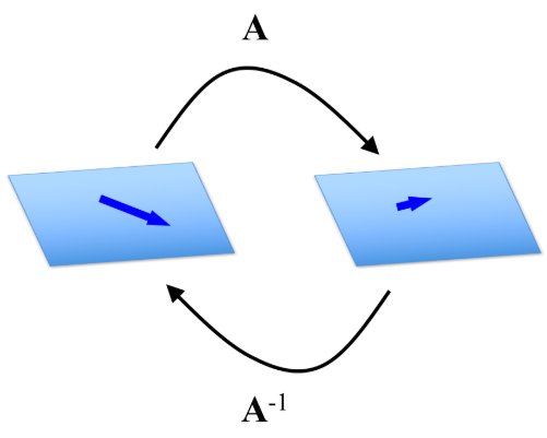
\( \det(A) \ne 0 \)

then the linear transformation \( L \) has an inverse transformation, denoted \( L^{-1} \).

The inverse transformation is given by

\( L^{-1}(\mathbf{v}) = A^{-1}\mathbf{v} \)

Applying \( L^{-1} \) reverses the effect of \( L \).

That is, for all vectors \( \mathbf{v} \in \mathbb{R}^2 \),

\( L^{-1}(L(\mathbf{v})) = \mathbf{v} \quad \text{and} \quad L(L^{-1}(\mathbf{v})) = \mathbf{v} \)

Thus, the inverse matrix represents the transformation that undoes the original transformation.

Example:

Let

\( A = \begin{pmatrix} 2 & 1 \\ 1 & 1 \end{pmatrix} \)

Find the inverse transformation.

▶️ Answer/Explanation

First compute the determinant:

\( \det(A) = (2)(1) – (1)(1) = 1 \ne 0 \)

So \( A \) is invertible. The inverse is

\( A^{-1} = \begin{pmatrix} 1 & -1 \\ -1 & 2 \end{pmatrix} \)

Conclusion: The inverse transformation is \( L^{-1}(\mathbf{v}) = A^{-1}\mathbf{v} \).

Example:

Explain why a linear transformation with determinant zero has no inverse.

▶️ Answer/Explanation

If \( \det(A) = 0 \), then \( A^{-1} \) does not exist.

Geometrically, the transformation collapses the plane into a line or a point, so the original vectors cannot be uniquely recovered.

Conclusion: Only linear transformations with nonzero determinant have inverses.

Scroll to Top