Modeling State Transitions with Matrices
In many contextual scenarios, quantities move between different states over time. These transitions are often described using percent changes.
A transition matrix can be constructed using these percent changes to model how the states evolve over discrete intervals, such as days, months, or years.
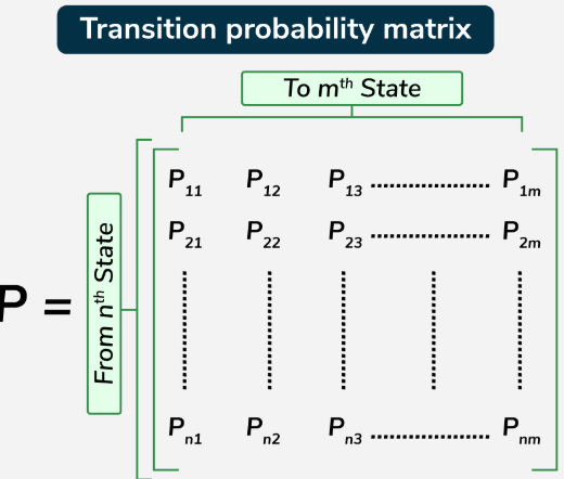
Each entry in the matrix represents the fraction (or percentage) of a quantity that moves from one state to another during one time step.
If the state vector at one time is written as
\( \mathbf{x}_n = \begin{pmatrix} x_1 \\ x_2 \end{pmatrix} \)
and the transition matrix is \( T \), then the state after one interval is given by
\( \mathbf{x}_{n+1} = T\mathbf{x}_n \)
Repeated multiplication models the system over multiple intervals.
Example:
A population is divided into two states: Urban and Rural.
Each year:
• 90% of the urban population remains urban, and 10% moves to rural.
• 20% of the rural population moves to urban, and 80% remains rural.
Construct the transition matrix.
▶️ Answer/Explanation
Write percentages as decimals and organize by destination:
\( T = \begin{pmatrix} 0.90 & 0.20 \\ 0.10 & 0.80 \end{pmatrix} \)
Conclusion: Multiplying this matrix by a state vector gives the population distribution after one year.
Example:
At the start of a year, a city has 600 urban residents and 400 rural residents. Use the transition matrix from the previous example to find the population after one year.
▶️ Answer/Explanation
Write the initial state vector:
\( \mathbf{x}_0 = \begin{pmatrix} 600 \\ 400 \end{pmatrix} \)
Multiply:
\( \mathbf{x}_1 = \begin{pmatrix} 0.90 & 0.20 \\ 0.10 & 0.80 \end{pmatrix} \begin{pmatrix} 600 \\ 400 \end{pmatrix} = \begin{pmatrix} 620 \\ 380 \end{pmatrix} \)
Final answer: After one year, there are 620 urban residents and 380 rural residents.
Steady State of a Transition Matrix
When a system is modeled using a transition matrix, repeatedly multiplying the matrix by the resulting state vectors can reveal the long-term behavior of the system.
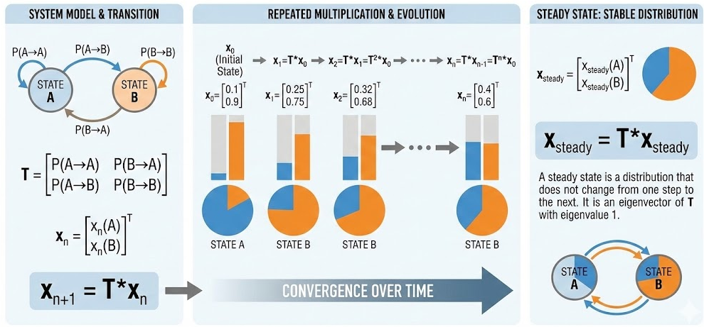
If \( T \) is a transition matrix and \( \mathbf{x}_n \) is the state vector after \( n \) steps, then
\( \mathbf{x}_{n+1} = T\mathbf{x}_n \)
As this process is repeated, the sequence of state vectors may approach a steady state.
A steady state is a distribution of values between states that does not change from one step to the next.
\( \mathbf{x}_{\text{steady}} = T\mathbf{x}_{\text{steady}} \)
This means the steady-state vector is an eigenvector of the transition matrix associated with the eigenvalue 1.
In many real-world contexts, the steady state represents long-term equilibrium behavior.
Example:
A system has two states, \( A \) and \( B \), with transition matrix
\( T = \begin{pmatrix} 0.75 & 0.40 \\ 0.25 & 0.60 \end{pmatrix} \)
Starting from an initial state vector, repeated multiplication produces the following vectors:
\( \mathbf{x}_1 = \begin{pmatrix} 520 \\ 480 \end{pmatrix}, \quad \mathbf{x}_2 = \begin{pmatrix} 510 \\ 490 \end{pmatrix}, \quad \mathbf{x}_3 = \begin{pmatrix} 505 \\ 495 \end{pmatrix} \)
Predict the steady state.
▶️ Answer/Explanation
The values are approaching a fixed distribution.
The steady state is approximately
\( \mathbf{x}_{\text{steady}} \approx \begin{pmatrix} 500 \\ 500 \end{pmatrix} \)
Conclusion: In the long run, the system stabilizes with equal distribution between the two states.
Example:
Explain how the steady state can be found without repeated multiplication.
▶️ Answer/Explanation
Solve the equation
\( \mathbf{x} = T\mathbf{x} \)
with the condition that the components sum to the total quantity or to 1 if using proportions.
Conclusion: The steady state corresponds to a fixed point of the transition matrix.
Using an Inverse Transition Matrix to Predict Past States
In some contextual models, transitions between states are represented by a transition matrix \( T \) such that
\( \mathbf{x}_{n+1} = T\mathbf{x}_n \)
If the transition matrix \( T \) is invertible, then it is possible to work backward to determine a previous state.
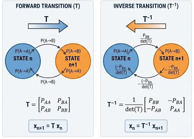
The inverse transition matrix, denoted \( T^{-1} \), satisfies
\( T^{-1}T = I \)
If the current state vector is \( \mathbf{x}_{n+1} \), then the previous state vector can be found by
\( \mathbf{x}_n = T^{-1}\mathbf{x}_{n+1} \)
This allows the model to predict past states, provided the transitions are reversible and accurately represented by the matrix.
This technique is useful in population studies, economics, and systems where historical distributions are unknown but current data is available.
Example:
A system has the transition matrix
\( T = \begin{pmatrix} 0.8 & 0.2 \\ 0.3 & 0.7 \end{pmatrix} \)
The current state vector is
\( \mathbf{x}_1 = \begin{pmatrix} 460 \\ 540 \end{pmatrix} \)
Find the previous state vector.
▶️ Answer/Explanation
First compute the determinant:
\( \det(T) = (0.8)(0.7) – (0.2)(0.3) = 0.56 – 0.06 = 0.50 \ne 0 \)
So the matrix is invertible. Its inverse is
\( T^{-1} = \begin{pmatrix} 1.4 & -0.4 \\ -0.6 & 1.6 \end{pmatrix} \)
Now multiply:
\( \mathbf{x}_0 = T^{-1}\mathbf{x}_1 = \begin{pmatrix} 1.4 & -0.4 \\ -0.6 & 1.6 \end{pmatrix} \begin{pmatrix} 460 \\ 540 \end{pmatrix} = \begin{pmatrix} 400 \\ 600 \end{pmatrix} \)
Final answer: The previous state was 400 in the first state and 600 in the second state.
Example:
Explain why predicting past states is not always possible.
▶️ Answer/Explanation
If the transition matrix is not invertible, then multiple past states may lead to the same current state.
In this case, information is lost and the past state cannot be uniquely determined.
Conclusion: Predicting past states requires an invertible transition matrix.