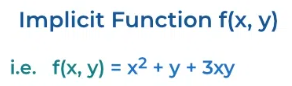
Implicitly Defined Functions
An equation involving two variables, typically written in the form \( F(x, y) = 0 \), can implicitly describe one or more functions.
In an implicit equation, the dependent variable is not isolated on one side of the equation. Instead, \( x \) and \( y \) are related together in a single equation.
Depending on the equation, it may be possible to solve for \( y \) in terms of \( x \), resulting in:
• one function
• more than one function
• or no function at all
Implicit equations are especially useful for describing curves such as circles, ellipses, and other relations that may fail the vertical line test.
Example:
Consider the equation
\( x^2 + y^2 = 9 \)
Determine the functions described by this equation.
▶️ Answer/Explanation
Solve for \( y \):
\( y^2 = 9 – x^2 \)
\( y = \pm \sqrt{9 – x^2} \)
This equation defines two functions:
\( y = \sqrt{9 – x^2} \) (upper semicircle)
\( y = -\sqrt{9 – x^2} \) (lower semicircle)
Conclusion: The implicit equation describes a circle, which corresponds to two functions of \( x \).
Example:
Consider the equation
\( y^3 + x = 0 \)
Determine whether this equation describes a function.
▶️ Answer/Explanation
Solve for \( y \):
\( y^3 = -x \)
\( y = \sqrt[3]{-x} \)
For each value of \( x \), there is exactly one value of \( y \).
Conclusion: This implicit equation defines a single function of \( x \).
Graphing Equations in Two Variables
An equation involving two variables can be graphed by finding pairs of values \( (x, y) \) that satisfy the equation.
Each solution \( (x, y) \) represents a point in the coordinate plane. The collection of all such points forms the graph of the equation.
Solutions can be found in several ways, including:
• Solving the equation for one variable in terms of the other
• Creating a table of values
• Identifying known geometric forms such as lines or circles
Some equations describe a single function, while others describe curves that represent multiple functions or relations.
Example:
Graph the equation
\( y = 2x – 1 \)
▶️ Answer/Explanation
Choose values of \( x \) and compute corresponding values of \( y \):
| \( x \) | \( y \) |
|---|---|
| 0 | -1 |
| 1 | 1 |
| 2 | 3 |
Plot the points and draw a straight line through them.
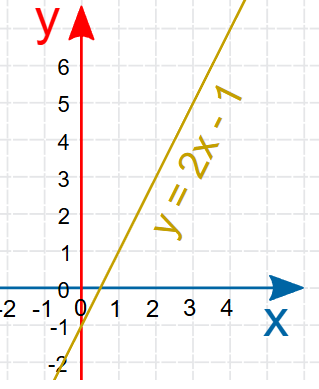
Conclusion: The graph is a straight line with slope 2 and y-intercept −1.
Example:
Graph the equation
\( x^2 + y^2 = 4 \)
▶️ Answer/Explanation
Solve for \( y \):
\( y = \pm \sqrt{4 – x^2} \)
This equation represents all points that are 2 units from the origin.
Plot points such as:
\( (2,0), (0,2), (-2,0), (0,-2) \)
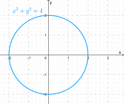
Conclusion: The graph is a circle of radius 2 centered at the origin.
Solving for a Variable to Define a Function
An equation involving two variables can sometimes be rewritten by solving for one variable in terms of the other.
When this is possible, the result defines a function whose graph is part or all of the graph of the original equation.
In such cases, the original equation may represent:
• a single function, or
• multiple functions corresponding to different branches of the graph
Each function obtained by solving for a variable corresponds to a portion of the original relation and may require a restricted domain.
Example:
Consider the equation
\( x^2 + y = 5 \)
Solve for \( y \) and describe the resulting function.
▶️ Answer/Explanation
Solve for \( y \):
\( y = 5 – x^2 \)
This defines a function of \( x \) whose graph is a downward-opening parabola.
Conclusion: The graph of the function \( y = 5 – x^2 \) is exactly the graph of the original equation.
Example:
Consider the equation
\( x^2 + y^2 = 9 \)
Solve for \( y \) and describe how the resulting functions relate to the graph.
▶️ Answer/Explanation
Solve for \( y \):
\( y = \pm \sqrt{9 – x^2} \)
This produces two functions:
\( y = \sqrt{9 – x^2} \), representing the upper semicircle
\( y = -\sqrt{9 – x^2} \), representing the lower semicircle
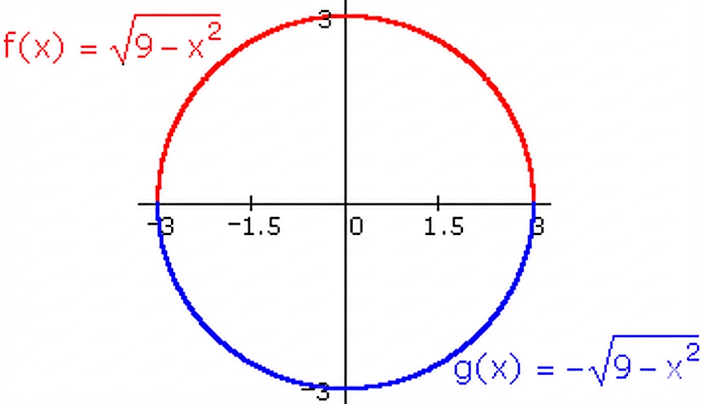
Conclusion: Each function corresponds to part of the original circle, and together they form the complete graph.
Sign of the Ratio of Changes for Implicitly Defined Functions
Consider an implicitly defined function represented by an equation involving two variables, such as \( F(x, y) = 0 \).
For two ordered pairs on the graph that are close together, the relationship between changes in the variables can be analyzed using the ratio
\( \dfrac{\Delta y}{\Delta x} \)
This ratio describes how \( y \) changes relative to \( x \) along the curve.
Positive ratio:
If \( \dfrac{\Delta y}{\Delta x} > 0 \), then \( x \) and \( y \) change in the same direction.
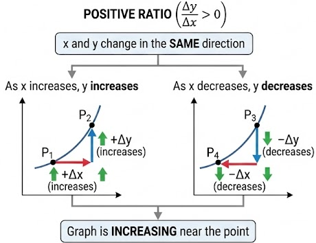
• As \( x \) increases, \( y \) increases
• As \( x \) decreases, \( y \) decreases
Negative ratio:
If \( \dfrac{\Delta y}{\Delta x} < 0 \), then \( x \) and \( y \) change in opposite directions.
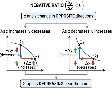
• As \( x \) increases, \( y \) decreases
• As \( x \) decreases, \( y \) increases
This local behavior helps describe whether the graph is increasing or decreasing near a given point, even when the function is not explicitly solved for one variable.
Example:
Consider the implicitly defined equation
\( y = x^2 \)
Describe how \( x \) and \( y \) change near \( x = 2 \).
▶️ Answer/Explanation
For points near \( x = 2 \), increasing \( x \) increases \( x^2 \).
Thus, \( \Delta x > 0 \) implies \( \Delta y > 0 \).
The ratio \( \dfrac{\Delta y}{\Delta x} \) is positive.
Conclusion: Near \( x = 2 \), both variables increase together.
Example:
Consider the implicitly defined equation
\( x^2 + y^2 = 25 \)
Describe how \( x \) and \( y \) change near the point \( (3, 4) \).
▶️ Answer/Explanation
Near \( (3,4) \), if \( x \) increases slightly, then \( x^2 \) increases.
To keep \( x^2 + y^2 = 25 \), \( y^2 \) must decrease, so \( y \) decreases.
Thus, \( \Delta x > 0 \) implies \( \Delta y < 0 \).
Conclusion: The ratio \( \dfrac{\Delta y}{\Delta x} \) is negative, so as one variable increases, the other decreases.
Zero Rates of Change and Horizontal or Vertical Behavior
For a relation or implicitly defined function involving two variables, the rate of change describes how one variable changes with respect to the other.
The rate of change of \( y \) with respect to \( x \) is given by
\( \dfrac{\Delta y}{\Delta x} \)
and the rate of change of \( x \) with respect to \( y \) is given by
\( \dfrac{\Delta x}{\Delta y} \)
Horizontal behavior occurs when the rate of change of \( y \) with respect to \( x \) is zero.
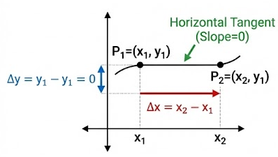
If \( \dfrac{\Delta y}{\Delta x} = 0 \), then \( y \) does not change as \( x \) changes, indicating a horizontal interval.
Vertical behavior occurs when the rate of change of \( x \) with respect to \( y \) is zero.
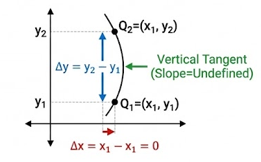
If \( \dfrac{\Delta x}{\Delta y} = 0 \), then \( x \) does not change as \( y \) changes, indicating a vertical interval.
These situations commonly occur at turning points, endpoints, or along curves such as circles and other implicitly defined relations.
Example:
Consider the function
\( y = x^2 \)
Describe the rate of change near \( x = 0 \).
▶️ Answer/Explanation
Near \( x = 0 \), small changes in \( x \) produce very small changes in \( y \).
At the point \( (0,0) \), the graph has a horizontal tangent.
This means \( \dfrac{\Delta y}{\Delta x} = 0 \), indicating a horizontal interval at that point.
Conclusion: The rate of change of \( y \) with respect to \( x \) is zero at the vertex of the parabola.
Example:
Consider the implicit equation
\( x^2 + y^2 = 16 \)
Describe the behavior near the point \( (4, 0) \).
▶️ Answer/Explanation
Near \( (4,0) \), changes in \( y \) cause almost no change in \( x \).
Thus, \( x \) remains approximately constant while \( y \) changes.
This means \( \dfrac{\Delta x}{\Delta y} = 0 \), indicating a vertical interval.
Conclusion: The circle has a vertical tangent at \( (4,0) \).