AP Statistics 1.10 The Investigative Question Revisited and Data Collection- Exam Style Questions - FRQs - New Syllabus

Question

A car maker produces four different models of cars: A, B, C, and D. A group of researchers is investigating which model of car has the longest distance traveled per gallon of gas (mileage). Higher mileage is considered better than lower mileage. The researchers will conduct a study in which they contact several owners of each model of car and ask them to estimate their mileage.

(a) Is this an observational study or an experiment? Justify your answer in context.

Model D has an autopilot feature, in which the car controls its own motion with human supervision. James owns a Model D car and will investigate whether using the autopilot feature results in higher mileage than not using the autopilot. James will drive his car on $70$ different days to and from work, using the same route at the same time each day. James will record the mileage each day.

(b) James will use a completely randomized design to conduct his investigation. Describe an appropriate method James could use to randomly assign the two treatments, driving using the autopilot feature and driving without using the autopilot feature, to $35$ days each.

(c) After the investigation was completed, James verified that the conditions for inference were met and conducted a hypothesis test. He discovered the mean mileage when using the autopilot feature was significantly higher than the mean mileage when not using the autopilot feature. James is a member of a Model D club with thousands of members who all drive Model D cars. He will give a presentation at a Model D club members’ meeting later this year and would like to state that the results of his hypothesis test apply to all Model D cars in his club. Another member of the club who is a statistician tells James his findings do not apply to all Model D cars in the club. What change would James need to make to his original study to be able to generalize to all Model D cars in the club?

Most-appropriate topic codes (AP Statistics):

• Topic $1.10$ — The Investigative Question Revisited and Data Collection (Parts $ \mathrm{a} $, $ \mathrm{c} $)
• Topic $1.13$ — Experimental Design (Part $ \mathrm{b} $)

▶️ Answer/Explanation

(a)
This is an observational study.
The researchers are simply gathering data by asking car owners to estimate their mileage, without actively imposing any treatments or randomly assigning participants to drive specific car models.

(b)
First, number the $70$ days from $1$ to $70$.
Write the numbers $1$ through $70$ on identical slips of paper, place them into a hat, and mix them thoroughly.
Draw $35$ slips of paper one by one without replacement.
The $35$ days corresponding to the drawn numbers will be assigned the treatment of driving with the autopilot feature, and the remaining $35$ days will be assigned to drive without the autopilot feature.

(c)
In order to generalize his findings to all Model D cars in his club, James cannot solely rely on an experiment conducted using only his own vehicle.
He would need to select a random sample of Model D cars (and their respective drivers) from the club’s membership to participate in his study.

Question

A developer wants to know whether adding fibers to concrete used in paving driveways will reduce the severity of cracking, because any driveway with severe cracks will have to be repaired by the developer. The developer conducts a completely randomized experiment with 60 new homes that need driveways. Thirty of the driveways will be randomly assigned to receive concrete that contains fibers, and the other 30 driveways will receive concrete that does not contain fibers. After one year, the developer will record the severity of cracks in each driveway on a scale of 0 to 10, with 0 representing not cracked at all and 10 representing severely cracked.

(a) Based on the information provided about the developer’s experiment, identify each of the following.

• Experimental units
• Treatments
• Response variable

(b) Describe an appropriate method the developer could use to randomly assign concrete that contains fibers and concrete that does not contain fibers to the 60 driveways.

Suppose the developer finds that there is a statistically significant reduction in the mean severity of cracks in driveways using the concrete that contains fibers compared to the driveways using concrete that does not contain fibers.

(c) In terms of the developer’s conclusion, what is the benefit of randomly assigning the driveways to either the concrete that contains fibers or the concrete that does not contain fibers?

Most-appropriate topic codes (AP Statistics):

• Topic $1.10$ — The Investigative Question Revisited and Data Collection (Part $ \mathrm{a} $)
• Topic $1.13$ — Experimental Design (Parts $ \mathrm{b} $, $ \mathrm{c} $)

▶️ Answer/Explanation

(a)
Experimental units: The 60 driveways (or the 60 new homes).
Treatments: The two types of concrete (concrete containing fibers and concrete without fibers).
Response variable: The severity of cracks in each driveway, measured on a scale of 0 to 10.

(b)
Number the 60 driveways from 1 to 60. Write the numbers 1 through 60 on identical slips of paper, place them in a hat, and mix thoroughly. Without looking, select 30 slips of paper one by one without replacement. The 30 driveways corresponding to the selected numbers will receive the concrete containing fibers, and the remaining 30 driveways will receive the concrete without fibers.

(c)
The primary benefit of random assignment is that it creates two treatment groups that are roughly equivalent at the beginning of the experiment. This helps to balance out the effects of potentially confounding variables, such as soil quality, driveway slope, or vehicle weight, across both groups. Because these other variables are distributed somewhat equally, the developer can confidently conclude that the statistically significant reduction in crack severity was actually caused by the addition of fibers to the concrete.

Question

A dermatologist will conduct an experiment to investigate the effectiveness of a new drug to treat acne. The dermatologist has recruited 36 pairs of identical twins. Each person in the experiment has acne and each person in the experiment will receive either the new drug or a placebo. After each person in the experiment uses either the new drug or the placebo for 2 weeks, the dermatologist will evaluate the improvement in acne severity for each person on a scale from 0 (no improvement) to 100 (complete cure).

(a) Identify the treatments, experimental units, and response variable of the experiment.

• Treatments:
• Experimental units:
• Response variable:

Each twin in the experiment has a severity of acne similar to that of the other twin. However, the severity of acne differs from one twin pair to another.

(b) For the dermatologist’s experiment, describe a statistical advantage of using a matched-pairs design where twins are paired rather than using a completely randomized design.

(c) For the dermatologist’s experiment, describe how the treatments can be randomly assigned to people using a matched-pairs design in which twins are paired.

Most-appropriate topic codes (AP Statistics):

• Topic $1.10$ — The Investigative Question Revisited and Data Collection (Part $ \mathrm{a} $)
• Topic $1.13$ — Experimental Design (Parts $ \mathrm{b} $, $ \mathrm{c} $)

▶️ Answer/Explanation

(a)
• Treatments: The new drug and the placebo.
• Experimental units: The 72 individual people (the 36 pairs of identical twins) participating in the experiment.
• Response variable: The improvement in acne severity, measured on a scale from 0 to 100.

(b)
A matched-pairs design controls for the variation in baseline acne severity and genetic/environmental factors among the subjects. Because identical twins share these traits, the difference in their acne improvement can be more directly attributed to the respective treatments rather than individual skin differences. This reduces the variability in the response and increases the statistical power to detect a true difference in effectiveness between the new drug and the placebo.

(c)
For each pair of identical twins, flip a fair coin. If the coin lands on heads, assign Twin A to receive the new drug and Twin B to receive the placebo. If the coin lands on tails, assign Twin A to receive the placebo and Twin B to receive the new drug. Repeat this random assignment process independently for all 36 pairs of twins.

Question

To compare success rates for treating allergies at two clinics that specialize in treating allergy sufferers, researchers selected random samples of patient records from the two clinics. The following table summarizes the data.

(a) (i) Complete the following table by recording the relative frequencies of successful and unsuccessful treatments at each clinic.

(ii) Based on the relative frequency table in part (a-i), which clinic is more successful in treating allergy sufferers? Justify your answer.

(b) Based on the design of the study, would a statistically significant result allow the researchers to conclude that receiving treatments at the clinic you selected in part (a-ii) causes a higher percentage of successful treatments than at the other clinic? Explain your answer.

A physician who worked at both clinics believed that it was important to separate the patients in the study by severity of the patient’s allergy (severe or mild). The physician constructed the following mosaic plot. The values in the mosaic plot represent the number of patients who were either successfully treated or unsuccessfully treated in each allergy severity group within each clinic. For example, the value 78 represents the number of patients successfully treated in the mild group within Clinic A.

Based on the mosaic plot, the physician concluded the following:
For mild allergy sufferers, Clinic B was more successful in treating allergies.
For severe allergy sufferers, Clinic B was more successful in treating allergies.

(c) (i) For each clinic, which allergy severity is treated more successfully? Justify your answer.

• Clinic A:
• Clinic B:

(ii) For each clinic, which allergy severity is more likely to be treated? Justify your answer.

• Clinic A:
• Clinic B:

(d) Using your answers from part (c), give a reasonable explanation of why the more successful clinic identified in part (a-ii) is the same as or different from the physician’s conclusion that Clinic B is more successful in treating both severe and mild allergies.

Most-appropriate topic codes (AP Statistics):

• Topic $1.10$ — The Investigative Question Revisited and Data Collection (Part $ \mathrm{b} $)
• Topic $2.1$ — Tabular and Graphical Representations for the Distributions of Two Categorical Variables (Parts $ \mathrm{a} $, $ \mathrm{c} $)
• Topic $2.2$ — Summary Statistics for Two Categorical Variables (Parts $ \mathrm{a} $, $ \mathrm{c} $, $ \mathrm{d} $)

▶️ Answer/Explanation

(a)(i)

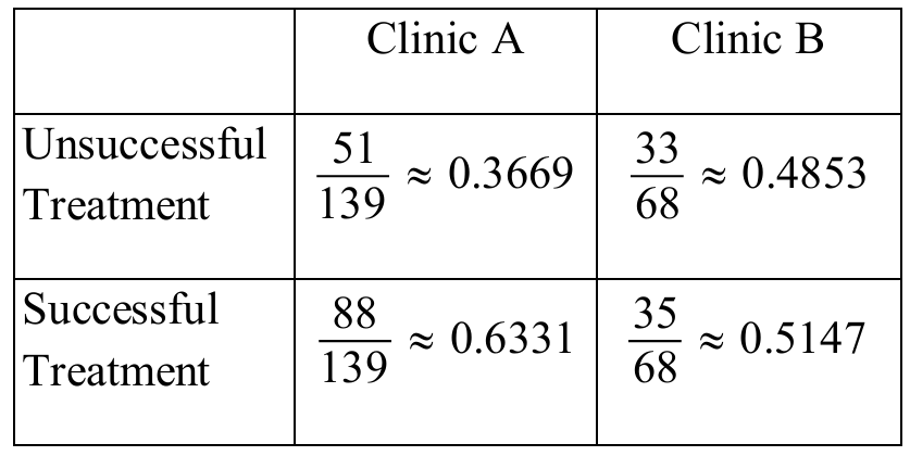
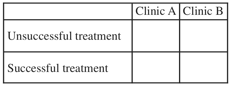
(a)(ii)
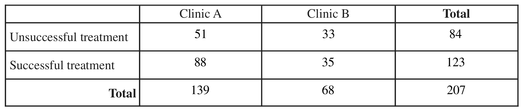
Clinic A is more successful. The relative frequency of successful treatments for Clinic A ($0.633$ or $63.3\%$) is greater than the relative frequency of successful treatments for Clinic B ($0.515$ or $51.5\%$).

(b)
No. The researchers selected random samples of patient records, which means this is an observational study, not a randomized experiment. Because patients were not randomly assigned to Clinic A or Clinic B, we cannot establish a cause-and-effect relationship due to the potential presence of confounding variables.

(c)(i)
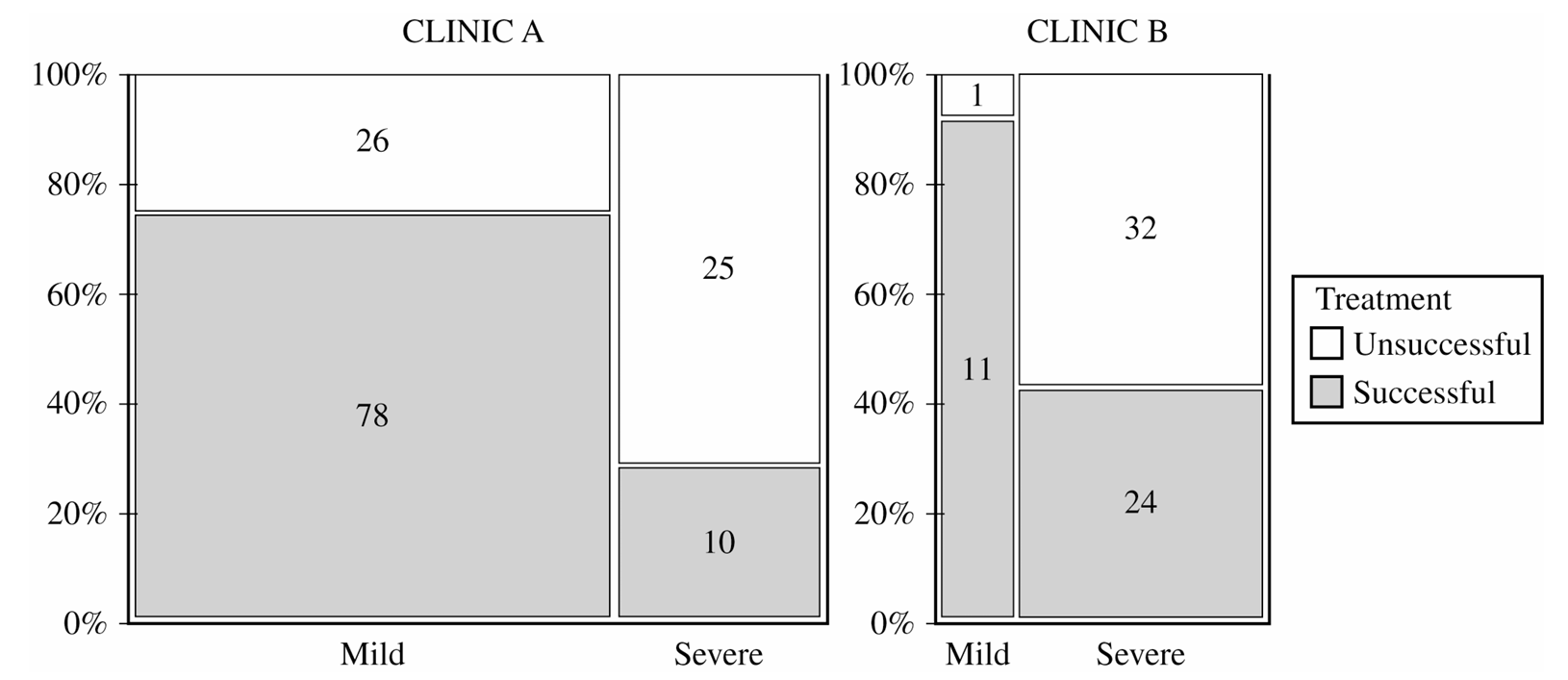
• Clinic A: Mild allergies are treated more successfully. The success rate for mild is $78 / (78 + 26) = 75\%$, while the success rate for severe is $11 / (11 + 24) = 31.4\%$.
• Clinic B: Mild allergies are treated more successfully. The success rate for mild is $32 / (32 + 1) = 97\%$, while the success rate for severe is $10 / (10 + 25) = 28.6\%$.

(c)(ii)
• Clinic A: Mild allergies are more likely to be treated. Clinic A treated 104 mild cases ($78+26$) compared to only 35 severe cases ($11+24$).
• Clinic B: Severe allergies are more likely to be treated. Clinic B treated 35 severe cases ($10+25$) compared to only 33 mild cases ($32+1$).

(d)
The conclusion is different because of Simpson’s Paradox. Clinic A’s overall success rate is higher because it treats a much larger proportion of mild allergy cases, which naturally have a higher success rate regardless of the clinic. Conversely, Clinic B treats a higher proportion of severe cases, which brings its overall average down, even though it performs better than Clinic A within each specific severity group.

Question

Researchers are investigating the effectiveness of using a fungus to control the spread of an insect that destroys trees.

The researchers will create four different concentrations of fungus mixtures: $0$ milliliters per liter ($\text{ml/L}$), $1.25\,\text{ml/L}$, $2.5\,\text{ml/L}$, and $3.75\,\text{ml/L}$.

An equal number of the insects will be placed into $20$ individual containers.

The group of insects in each container will be sprayed with one of the four mixtures, and the researchers will record the number of insects that are still alive in each container one week after spraying.

(a) Identify the treatments, experimental units, and response variable of the experiment.

Treatments:

Experimental units:

Response variable:

(b) Does the experiment have a control group? Explain your answer.

(c) Describe how the treatments can be randomly assigned to the experimental units so that each treatment has the same number of units.

Most-appropriate topic codes (AP Statistics):

• Topic $1.10$ — The Investigative Question Revisited and Data Collection (Parts $ \mathrm{a} $, $ \mathrm{b} $)
• Topic $1.13$ — Experimental Design (Part $ \mathrm{c} $)

▶️ Answer/Explanation

(a)
Treatments: The four different concentrations of the fungus spray ($0\,\text{ml/L}$, $1.25\,\text{ml/L}$, $2.5\,\text{ml/L}$, and $3.75\,\text{ml/L}$).
Experimental units: The $20$ individual containers, each containing an equal number of insects.
Response variable: The number of insects that are still alive in each container one week after being sprayed.

(b)
Yes, the experiment definitely has a control group.
The containers sprayed with the $0\,\text{ml/L}$ concentration form the control group because this specific mixture contains absolutely no fungus, serving as a baseline for comparison.

(c)
First, label each of the $20$ containers with a unique integer from $1$ to $20$.
Next, use a random number generator to select $15$ unique integers from $1$ to $20$ without replacement.
Assign the first five containers selected to receive the $0\,\text{ml/L}$ treatment.
Assign the next five containers selected to receive the $1.25\,\text{ml/L}$ treatment, and the next five to receive the $2.5\,\text{ml/L}$ treatment.
Finally, the remaining five containers that were not selected will automatically receive the $3.75\,\text{ml/L}$ treatment.

Question

Alzheimer’s disease results in a loss of cognitive ability beyond what is expected with typical aging. A local newspaper published an article with the following headline.

Study Finds Strong Association Between Smoking and Alzheimer’s

The article reported that a study tracked the medical histories of 21,123 men and women for 23 years. The article stated that, for those who smoked at least two packs of cigarettes a day, the risk of developing Alzheimer’s disease was 2.57 times the risk for those who did not smoke.

(a) Identify the explanatory and response variables in the study.

Explanatory variable:

Response variable:

(b) Is the study described in the article an observational study or an experiment? Explain.

(c) Exercise status (regular weekly exercise versus no regular weekly exercise) was mentioned in the article as a possible confounding variable. Explain how exercise status could be a confounding variable in the study.

Most-appropriate topic codes (AP Statistics):

• Topic $1.10$ — The Investigative Question Revisited and Data Collection (Parts $ \mathrm{a} $, $ \mathrm{b} $)
• Topic $1.11$ — Random Smapling (Part $ \mathrm{b} $)
• Topic $1.12$ — Potential Problems with Sampling (Part $ \mathrm{c} $)

▶️ Answer/Explanation

(a)

Explanatory variable: The person’s degree of cigarette smoking — specifically, whether or not the individual smoked at least two packs of cigarettes per day (smoker of at least two packs per day versus non-smoker at that level).
Response variable: Whether or not the person developed Alzheimer’s disease during the course of the 23-year study.

(b)

This is an observational study, not an experiment. In an experiment, researchers would have to actively assign the treatment — in this case, the level of cigarette smoking — to the participants. Instead, the researchers simply tracked the existing medical histories of 21,123 men and women over 23 years. The smoking status of each person was passively observed and recorded, not controlled or manipulated by the researchers. Since no treatment was imposed, this is an observational study.

(c)

A confounding variable is one that is related to the explanatory variable and also independently influences the response variable, making it difficult to determine whether the explanatory variable alone is responsible for the observed association.
Exercise status could be a confounding variable here for two reasons working together:
First, people who exercise regularly tend to be more health-conscious overall, and as a result are less likely to smoke heavily. So exercise status is related to the explanatory variable — smoking status. Heavy smokers are, on average, less likely to exercise regularly than non-smokers.
Second, regular exercise may independently reduce the risk of developing Alzheimer’s disease. So exercise status is also related to the response variable — development of Alzheimer’s disease.
Because of both of these relationships, the observed association between heavy smoking and higher rates of Alzheimer’s could be at least partly explained by the fact that heavy smokers tend to exercise less — and it is the lack of exercise, not the smoking itself, that contributes to the increased risk. This makes it impossible to determine from this study alone whether the association between smoking and Alzheimer’s reflects a true causal relationship or is merely the result of exercise status being linked to both.

Question

To determine the amount of sugar in a typical serving of breakfast cereal, a student randomly selected 60 boxes of different types of cereal from the shelves of a large grocery store.

The student noticed that the side panels of some of the cereal boxes showed sugar content based on one-cup servings, while others showed sugar content based on three-quarter-cup servings. Many of the cereal boxes with side panels that showed three-quarter-cup servings were ones that appealed to young children, and the student wondered whether there might be some difference in the sugar content of the cereals that showed different-size servings on their side panels. To investigate the question, the data were separated into two groups. One group consisted of 29 cereals that showed one-cup serving sizes; the other group consisted of 31 cereals that showed three-quarter-cup serving sizes. The boxplots shown below display sugar content (in grams) per serving of the cereals for each of the two serving sizes.

(a) Write a few sentences to compare the distributions of sugar content per serving for the two serving sizes of cereals.

After analyzing the boxplots on the preceding page, the student decided that instead of a comparison of sugar content per recommended serving, it might be more appropriate to compare sugar content for equal-size servings. To compare the amount of sugar in serving sizes of one cup each, the amount of sugar in each of the cereals showing three-quarter-cup servings on their side panels was multiplied by $\dfrac{4}{3}$. The bottom boxplot shown below displays sugar content (in grams) per cup for those cereals that showed a serving size of three-quarter-cup on their side panels.

(b) What new information about sugar content do the boxplots above provide?

(c) Based on the boxplots shown above on this page, how would you expect the mean amounts of sugar per cup to compare for the different recommended serving sizes? Explain.

Most-appropriate topic codes (AP Statistics):

• Topic $1.1$ — Analyzing Categorical Data / Representing Data Graphically (Parts $\mathrm{a}$, $\mathrm{b}$)
• Topic $1.7$ — Summary Statistics for a Quantitative Variable (Center, Spread, Shape) (Parts $\mathrm{a}$, $\mathrm{b}$, $\mathrm{c}$)
• Topic $1.9$ — Comparing Distributions of a Quantitative Variable (Parts $\mathrm{a}$, $\mathrm{b}$)
• Topic $1.10$ — The Effect of Adding a Constant or Multiplying by a Constant on Summary Statistics (Part $\mathrm{b}$)
• Topic $3.1$ — Mean and Standard Deviation of a Linear Transformation (Part $\mathrm{c}$)

▶️ Answer/Explanation

(a)

When comparing two distributions from boxplots, we examine center, spread, shape, and unusual features.
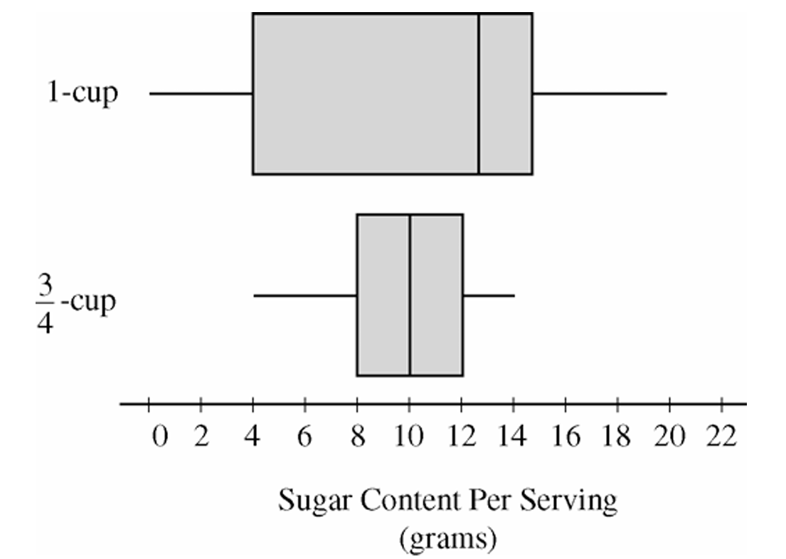
The cereals with one-cup serving sizes have a higher median sugar content per serving than the cereals with three-quarter-cup serving sizes. The one-cup distribution also has greater variability, as indicated by its larger range and larger interquartile range (IQR). In terms of shape, the one-cup distribution appears somewhat left-skewed because the median is closer to the upper quartile than to the lower quartile, while the three-quarter-cup distribution is more nearly symmetric. Neither distribution appears to contain extreme outliers.

(b)

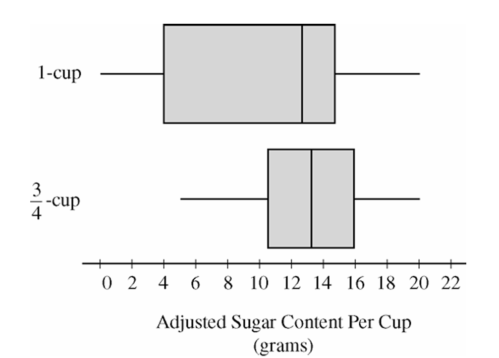
Multiplying each sugar value in the three-quarter-cup group by $\dfrac{4}{3}$ converts the measurements to sugar content per cup, allowing a fair comparison using equal serving sizes.
The adjusted boxplot shows that cereals with recommended serving sizes of three-quarter cup tend to contain more sugar per cup than cereals with recommended serving sizes of one cup. The median for the adjusted three-quarter-cup distribution is now noticeably higher than the median for the one-cup distribution. In addition, all measures of spread (range and IQR) for the adjusted distribution have increased by a factor of $\dfrac{4}{3}$, reflecting the effect of multiplying every observation by a constant.

(c)

We would expect the mean sugar content per cup to be greater for cereals that list a serving size of three-quarter cup.
After adjustment, the three-quarter-cup distribution has a higher center than the one-cup distribution, as seen from its higher median. Because the mean generally follows the center of the distribution, the higher overall location of the adjusted three-quarter-cup distribution suggests a larger mean sugar content per cup.
$\boxed{\bar{x}_{\frac{3}{4}\text{-cup}} > \bar{x}_{\text{1-cup}}}$

Question

As dogs age, diminished joint and hip health may lead to joint pain and thus reduce a dog’s activity level. Such a reduction in activity can lead to other health concerns such as weight gain and lethargy due to lack of exercise. A study is to be conducted to see which of two dietary supplements, glucosamine or chondroitin, is more effective in promoting joint and hip health and reducing the onset of canine osteoarthritis. Researchers will randomly select a total of 300 dogs from ten different large veterinary practices around the country. All of the dogs are more than 6 years old, and their owners have given consent to participate in the study. Changes in joint and hip health will be evaluated after 6 months of treatment.

(a) What would be an advantage to adding a control group in the design of this study?

(b) Assuming a control group is added to the other two groups in the study, explain how you would assign the 300 dogs to these three groups for a completely randomized design.

(c) Rather than using a completely randomized design, one group of researchers proposes blocking on clinics, and another group of researchers proposes blocking on breed of dog. How would you decide which one of these two variables to use as a blocking variable?

Most-appropriate topic codes (AP Statistics):

• Topic 1.13 — Experimental Design (Parts $\mathrm{a}$, $\mathrm{b}$, $\mathrm{c}$)
• Topic 1.10 — The Investigative Question Revisited and Data Collection (Part $\mathrm{a}$)
• Topic 1.11 — Random Sampling (Part $\mathrm{b}$)

▶️ Answer/Explanation

(a)

A control group gives the researchers a baseline comparison group — without any dietary supplement — so they can measure whether glucosamine or chondroitin actually makes a difference beyond what would happen due to the normal aging process alone.
Without a control group, we could not tell whether any improvements in joint and hip health were caused by the supplements or simply by other factors such as the passage of time, veterinary care, or natural variation between dogs.
In this study specifically, the control group allows us to isolate the true effect of glucosamine and chondroitin on reducing canine osteoarthritis by comparing both treatment groups against untreated dogs under the same conditions.
$\boxed{\text{Control group provides a baseline to determine whether the supplements are truly effective.}}$

(b)

First, assign each of the 300 dogs a unique number from $001$ to $300$.
Then, use a random number generator (calculator, statistical software, or a random number table) to randomly select 100 numbers from $001$ to $300$, ignoring any repeats — the dogs corresponding to these 100 numbers are assigned to the glucosamine group.
From the remaining 200 dogs, randomly select another 100 numbers using the same process — these dogs are assigned to the chondroitin group.
The final 100 remaining dogs are assigned to the control group and receive no dietary supplement.
$\boxed{\text{Randomly assign dogs numbered } 001\text{–}300 \text{ into three equal groups of 100 using a random number generator.}}$

(c)

The blocking variable should be the one that has a stronger association with the response variable — joint and hip health — so that dogs within each block are as similar (homogeneous) as possible.
Breed of dog is associated with the size of the dog, and size is known to be related to joint and hip health — larger breeds tend to have more joint problems than smaller breeds, so breed is likely to create more variability in the response.
Clinic, on the other hand, is less likely to be strongly associated with joint and hip health because most large veterinary practices see a wide variety of dog breeds and sizes, so dogs across clinics would not be meaningfully more similar to each other than dogs across breeds.
Therefore, we should block on breed of dog, since it is more strongly related to joint and hip health and will reduce variability more effectively within each block.
$\boxed{\text{Block on breed of dog, as it has a stronger relationship to joint and hip health than clinic.}}$

Question

The goal of a nutritional study was to compare the caloric intake of adolescents living in rural areas of the United States with the caloric intake of adolescents living in urban areas of the United States. A random sample of ninth-grade students from one high school in a rural area was selected. Another random sample of ninth graders from one high school in an urban area was also selected. Each student in each sample kept records of all the food he or she consumed in one day.

The back-to-back stemplot below displays the number of calories of food consumed per kilogram of body weight for each student on that day.

(a) Write a few sentences comparing the distribution of the daily caloric intake of ninth-grade students in the rural high school with the distribution of the daily caloric intake of ninth-grade students in the urban high school.

(b) Is it reasonable to generalize the findings of this study to all rural and urban ninth-grade students in the United States? Explain.

(c) Researchers who want to conduct a similar study are debating which of the following two plans to use.

Plan I: Have each student in the study record all the food he or she consumed in one day. Then researchers would compute the number of calories of food consumed per kilogram of body weight for each student for that day.

Plan II: Have each student in the study record all the food he or she consumed over the same 7-day period. Then researchers would compute the average daily number of calories of food consumed per kilogram of body weight for each student during that 7-day period.

Assuming that the students keep accurate records, which plan, I or II, would better meet the goal of the study? Justify your answer.

Most-appropriate topic codes (AP Statistics):

• Topic 1.9 — Comparisons of the Distributions for One Quantitative Variable (Part $\mathrm{a}$)
• Topic 1.11 — Random Sampling (Part $\mathrm{b}$)
• Topic 1.12 — Potential Problems with Sampling (Part $\mathrm{b}$)
• Topic 1.10 — The Investigative Question Revisited and Data Collection (Part $\mathrm{c}$)

▶️ Answer/Explanation

(a)
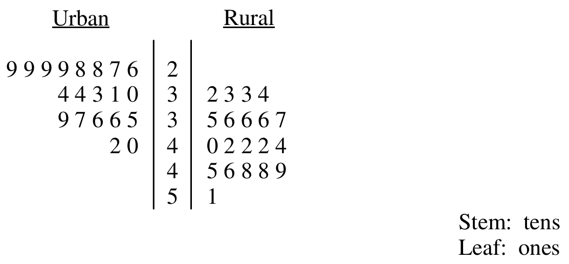
Reading the stemplot, the rural distribution is centered higher and is more spread out than the urban distribution.

For the rural students:

Mean $\approx 40.45$ cal/kg
Median $\approx 41$ cal/kg
Range $= 19$
SD $\approx 6.04$
IQR $\approx 10$

For the urban students:

Mean $\approx 32.6$ cal/kg
Median $\approx 32$ cal/kg
Range $= 16$
SD $\approx 4.67$
IQR $\approx 7$

So both the typical value and the spread are larger for the rural group. In terms of shape, the rural data look fairly symmetric and spread evenly between about 32 and 51 cal/kg, while the urban data appear skewed toward the larger values.

$ \boxed{\text{Rural: higher center and more spread; Urban: lower center, less spread, right-skewed}} $

(b)
No. Each sample came from just one rural school and one urban school, so these two specific schools may not represent the much larger and more diverse population of all rural and urban ninth graders across the country. Because the schools themselves were not randomly chosen from all such schools, the results can’t be safely extended beyond these two schools.

$ \boxed{\text{No — only one school of each type was sampled, so results cannot be generalized nationally}} $

(c)
Plan II is the better choice.

Both plans already adjust for body size by dividing calories by body weight, so that part is the same. The real issue is that a single day’s eating can be unusually high or low depending on what happened that day — a birthday party, a sick day, a weekend versus a school day, and so on. By recording food over a full 7-day period and averaging, Plan II smooths out this day-to-day variability and gives a more stable, precise picture of each student’s typical caloric intake.

$ \boxed{\text{Plan II — averaging over 7 days reduces day-to-day variability and gives a more precise estimate}} $

Question

Researchers who are studying a new shampoo formula plan to compare the condition of hair for people who use the new formula with the condition of hair for people who use the current formula. Twelve volunteers are available to participate in this study. Information on these volunteers (numbered 1 through 12) is shown in the table below.

(a) These researchers want to conduct an experiment involving the two formulas (new and current) of shampoo. They believe that the condition of hair changes with age but not gender. Because researchers want the size of the blocks in an experiment to be equal to the number of treatments, they will use blocks of size 2 in their experiment. Identify the volunteers (by number) that would be included in each of the six blocks and give the criteria you used to form the blocks.

(b) Other researchers believe that hair condition differs with both age and gender. These researchers will also use blocks of size 2 in their experiment. Identify the volunteers (by number) that would be included in each of the six blocks and give the criteria you used to form the blocks.

(c) The researchers in part (b) decide to select three of the six blocks to receive the new formula and to give the other three blocks the current formula. Is this an appropriate way to assign treatments? If so, describe a method for selecting the three blocks to receive the new formula. If not, describe an appropriate method for assigning treatments.

Most-appropriate topic codes (AP Statistics):

• Topic 1.13 — Experimental Design (Parts a, b, c)
• Topic 1.10 — The Investigative Question Revisited and Data Collection (Parts a, b)

▶️ Answer/Explanation

(a)
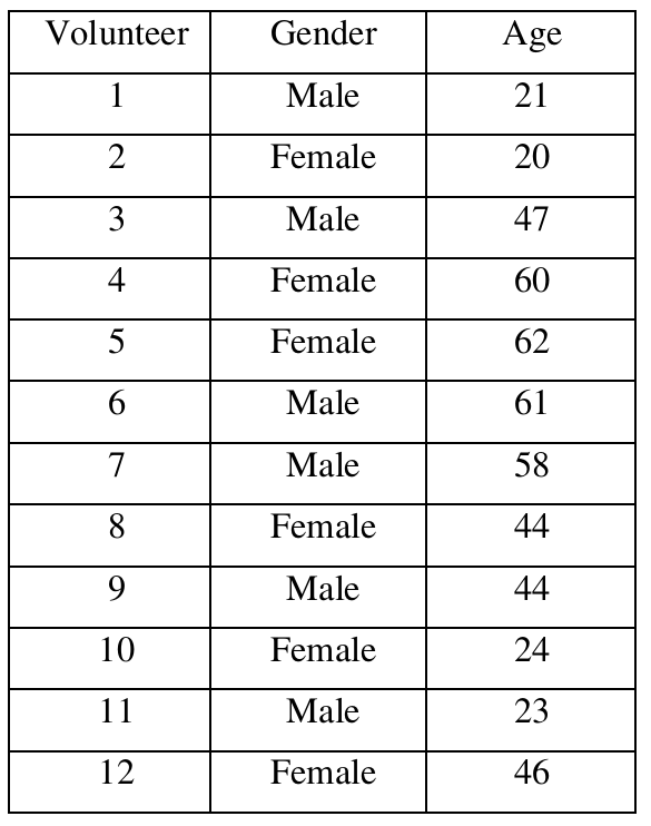
Pairing consecutive volunteers by age (without regard to gender) gives the six blocks:

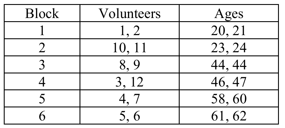
Since these researchers believe that the condition of hair changes with age but not gender, the volunteers are sorted from youngest to oldest. The volunteers in the sorted list are paired to form six blocks of size two. More specifically, the youngest two volunteers are placed in the first block. The next two volunteers in the sorted list are placed in the second block. This pairing continues until all six blocks of two are formed, with the oldest two volunteers in the sixth block.

(b)
Since both age and gender are believed to affect hair condition, volunteers must be blocked so that each block contains two people of the same gender and similar age.
First, separate by gender, then sort each group by age and pair consecutively
Males sorted by age: Volunteer 1 (age 21), Volunteer 11 (age 23), Volunteer 9 (age 44), Volunteer 3 (age 47), Volunteer 7 (age 58), Volunteer 6 (age 61)
Females sorted by age: Volunteer 2 (age 20), Volunteer 10 (age 24), Volunteer 8 (age 44), Volunteer 12 (age 46), Volunteer 4 (age 60), Volunteer 5 (age 62)
The six blocks are:

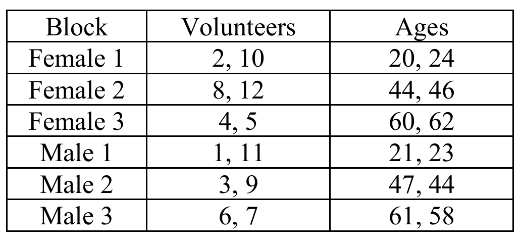
Since these researchers believe that the condition of hair changes with both age and gender, the women are sorted from youngest to oldest and then the men are sorted from youngest to oldest. The women (men) in the sorted list are paired to form the blocks of size two. More specifically, the youngest two women (men) are placed in a block. The next two youngest women (men) are placed in another block. Finally, the oldest two women (men) are placed in another block.

(c)
No, this is not an appropriate method for assigning treatments. Assigning the new formula to three entire blocks and the current formula to three other blocks does not allow a fair within-block comparison, because within each block both members would receive the same formula.
The correct approach in a matched-pairs block design is to randomly assign one person within each block to the new formula and the other to the current formula. This can be done as follows:
For each of the six blocks, flip a fair coin (or use a random number table/generator). If the result is heads (or the random digit is 0–4), assign the lower-numbered volunteer to the new formula and the other to the current formula. If tails (or digit 5–9), reverse the assignment. This ensures that within every block, one person receives the new formula and one receives the current formula, making a valid matched comparison possible.
$\boxed{\text{Randomly assign one person per block to new formula; other receives current formula}}$

AP Statistics 1.10 The Investigative Question Revisited and Data Collection- Exam Style Questions - FRQs - New Syllabus

Question

Question

Question

Question

Question

Question

Question

Question

Question

Question

Resources

Members

Company