
AP Statistics 1.12 Potential Problems with Sampling- Exam Style Questions - FRQs - New Syllabus
Question
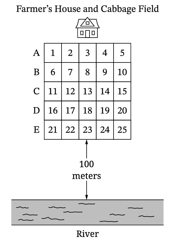
- Sampling method I: Select region 3, which is closest to the farmer’s house and farthest from the river. Examine every cabbage plant in the region for aphid damage.
- Sampling method II: Randomly select one row (A, B, C, D, or E). For every region in the selected row, examine every cabbage plant for aphid damage.
- Sampling method III: Randomly select one region from each of rows A, B, C, D, and E. For each selected region, examine every cabbage plant for aphid damage.
Most-appropriate topic codes (AP Statistics):
• Topic \(1.12\) — Potential Problems with Sampling (Parts \( \mathrm{A} \), \( \mathrm{B} \))
▶️ Answer/Explanation
A.
• Sampling method I is not an appropriate sampling method because it uses a convenience sample that lacks randomization.
• Since region 3 is located farthest from the river where aphid damage is believed to be lowest, this region is not representative of the whole field and will likely lead to an underestimate of the true population proportion.
B.
• The selection of row E is likely to provide an overestimate of the true proportion of damaged cabbage plants.
• Row E is the row positioned closest to the river, meaning every single plant checked in this sample belongs to the high-risk zone where the farmer expects aphid damage to be at its peak concentration.
C.
• Label the 5 individual regions within row A with unique identifiers from 1 to 5.
• Use a random number generator or draw numbered slips from a hat to select one single region from row A.
• Repeat this exact independent drawing process for row B (regions 6 to 10), row C (regions 11 to 15), row D (regions 16 to 20), and row E (regions 21 to 25) to complete a stratified sample containing exactly 5 distinct regions.
Question
Most-appropriate topic codes (AP Statistics):
• Topic \(1.12\) — Potential Problems with Sampling (Part \( \mathrm{a} \))
▶️ Answer/Explanation
(a)
Keeping a daily journal introduces response bias because subjects are self-reporting. They might forget to log short walks or underestimate their distances, which would cause our sample’s average daily miles to be systematically biased too low compared to what they actually walked.
(b)
A representative sample is essential because it allows us to generalize our findings. By selecting randomly, our \(100\) adults look like the larger target population, meaning any inference we make about the relationship between walking and cholesterol isn’t skewed by an unrepresentative group.
(c)
No, we can’t claim causation here because this is an observational study, not an experiment. We didn’t randomly assign subjects to walk specific distances. Because of this lack of assignment, there could be confounding variables at play—like a person’s diet or general health consciousness—that simultaneously affect both how much they walk and their cholesterol levels.
Question
• Calculate and record the median of the sample.
• Repeat the process to obtain a total of \(15,000\) medians.
Most-appropriate topic codes (AP Statistics):
• Topic \(1.12\) — Potential Problems with Sampling (Part \( \mathrm{a} \))
• Topic \(1.7\) — Summary Statistics for One Quantitative Variable (Parts \( \mathrm{b} \), \( \mathrm{d} \), \( \mathrm{e} \))
• Topic \(2.12\) — Central Limit Theorem and Sampling Distributions for Sample Means (Parts \( \mathrm{c} \), \( \mathrm{f} \))
▶️ Answer/Explanation
(a)
Because a random sample was used, it is appropriate to generalize the results to the population of all rental prices for one-bedroom apartments in the city that are listed on this particular website at the time the sample was taken.
(b)
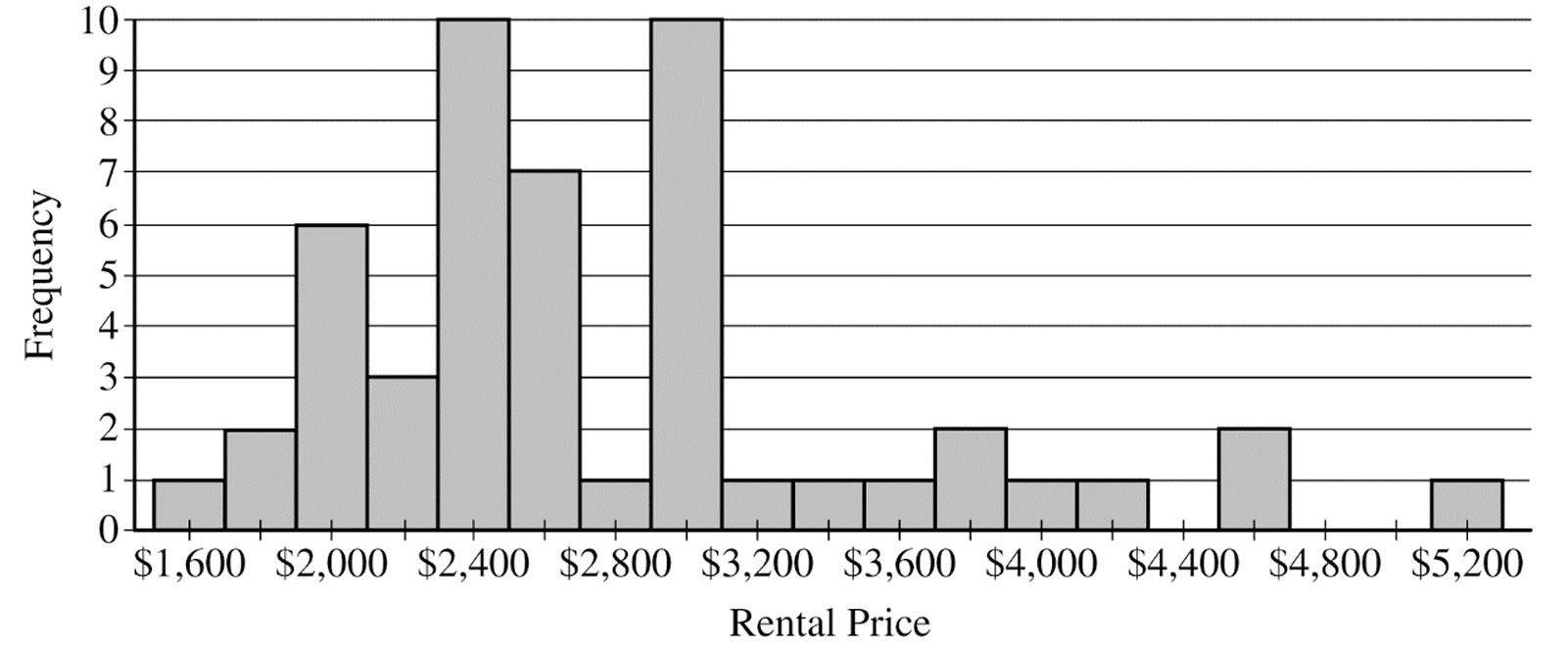
The histogram indicates that the distribution of rental prices is strongly skewed to the right.
Because of this right skewness, the sample mean will be pulled substantially higher by a few very large rental prices.
Consequently, the sample mean would overestimate the typical rental price, whereas the sample median provides a more accurate representation of the center.
(c)
To develop a theoretical sampling distribution, Emma would need to obtain every possible sample of size \(50\) from the population of apartments listed on the website.
She would then compute the median rental price for each of these possible samples.
The entire collection of all these computed sample medians forms the theoretical sampling distribution for the sample median.
(d)
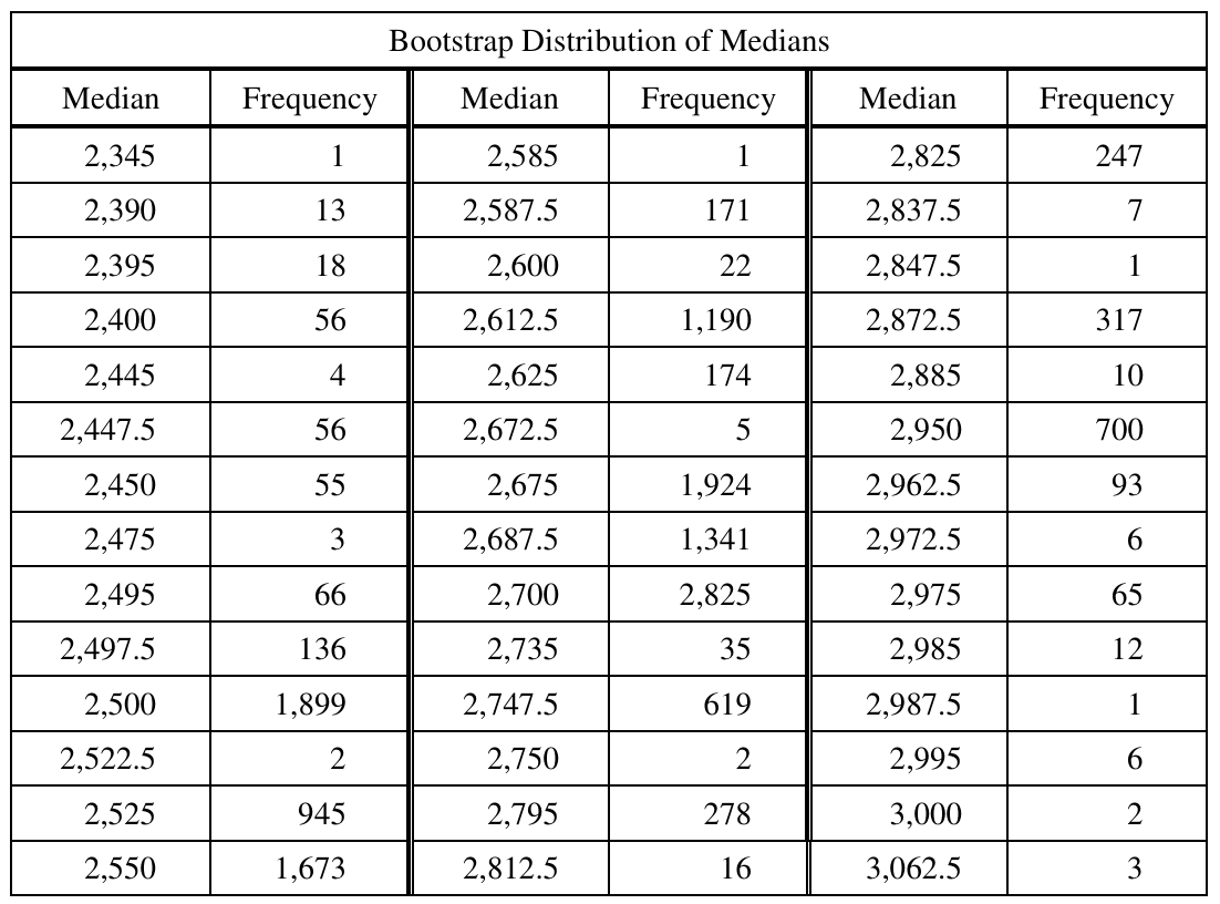
i. The \(5\text{th}\) percentile corresponds to the \((0.05)(15,000) = 750\text{th}\) value in the ordered data.
By keeping a running cumulative total of the frequencies down the columns, the \(750\text{th}\) value first falls in the row for the median of \(\$2,500\).
ii. The \(95\text{th}\) percentile corresponds to the \((0.95)(15,000) = 14,250\text{th}\) value in the ordered data.
Continuing to add the frequencies, the \(14,250\text{th}\) value falls in the row for the median of \(\$2,950\).
(e)
We need to sum the frequencies of all bootstrap medians from \(\$2,500\) to \(\$2,950\) inclusive.
\(\text{Sum} = 1,899 + 2 + \dots + 10 + 700 = 14,404\)
\(\text{Percentage} = \left(\dfrac{14,404}{15,000}\right) \times 100\% \approx 96.03\%\)
(f)
Based on our previous parts, an approximate \(96\%\) confidence interval for the median is \((\$2,500, \$2,950)\).
Interpretation: We are approximately \(96\%\) confident that the true median rental price of all one-bedroom apartments listed on this website for this city is between \(\$2,500\) and \(\$2,950\).
Question
If heads, you must respond no, regardless of whether you regularly recycle. If tails, please truthfully respond yes or no.
Most-appropriate topic codes (AP Statistics):
• Topic \(2.6\) — Conditional Probability (Part \( \mathrm{c}\text{-}\mathrm{ii} \))
• Topic \(2.8\) — Introduction to Random Variables and Probability Distributions (Part \( \mathrm{c}\text{-}\mathrm{i} \))
• Topic \(3.3\) — Constructing a Confidence Interval for a Population Proportion (Part \( \mathrm{a} \))
▶️ Answer/Explanation
(a)
The sample selected by the environmental science teacher contained $60$ students.
Detailed Solution:
First, find the point estimate $\hat{p}$ which is the midpoint of the confidence interval: $\hat{p} = \frac{0.584 + 0.816}{2} = 0.70$.
Next, determine the margin of error ($ME$) by calculating the distance from the midpoint to an endpoint: $ME = 0.816 – 0.70 = 0.116$.
Using the margin of error formula $ME = z^* \sqrt{\frac{\hat{p}(1-\hat{p})}{n}}$ for a $95\%$ confidence level ($z^* = 1.96$), we set up the equation $0.116 = 1.96 \sqrt{\frac{0.70(1-0.70)}{n}}$.
Solving for $n$ gives us $\sqrt{n} = \frac{1.96 \sqrt{0.21}}{0.116} \approx 7.74$, which squares to $n \approx 59.9$, revealing that the teacher’s sample size is exactly $60$ students.
(b)
Bias might have been introduced because students were asked directly by their environmental science teacher, which likely creates response bias.
Detailed Solution:
Because the survey is conducted face-to-face by a teacher who is expected to care about the environment, students may feel strong social pressure to give the “desirable” answer.
This phenomenon is known as response bias, where respondents do not answer truthfully in order to avoid judgment or please the interviewer.
As a result, more students will claim they recycle than actually do, artificially inflating the number of “yes” responses and causing the point estimate to be higher than the true population proportion.
(c)(i)
The expected number of students required to respond “no” due to the coin flip is $150$.
Detailed Solution:
Since the students are flipping a fair coin, the theoretical probability of getting heads is exactly $0.5$.
With a total random sample of $n = 300$ students, the expected number of heads is calculated as $n \times p = 300 \times 0.5$.
Therefore, we can expect exactly half the students, or $150$, to be forced to respond “no” based on the coin flip instructions.
(c)(ii)
The point estimate for the proportion of all students at the high school who would respond “yes” is $0.58$.
Detailed Solution:
Out of the $300$ total students, $213$ responded “no”, and we expect $150$ of these “no” responses to come from the students who flipped heads.
This means the remaining $213 – 150 = 63$ “no” responses came from the $150$ students who flipped tails and answered truthfully about not recycling.
Since $150$ students flipped tails and $63$ of them truthfully said “no”, the remaining $150 – 63 = 87$ students must have truthfully answered “yes”.
Thus, the point estimate for the proportion of students who actually recycle is $\frac{87}{150} = 0.58$.
Question
Most-appropriate topic codes (AP Statistics):
• Topic \(1.11\) — Random Smapling (Part \( \mathrm{b} \))
• Topic \(1.12\) — Potential Problems with Sampling (Part \( \mathrm{c} \))
▶️ Answer/Explanation
(a)
Explanatory variable: The person’s degree of cigarette smoking — specifically, whether or not the individual smoked at least two packs of cigarettes per day (smoker of at least two packs per day versus non-smoker at that level).
Response variable: Whether or not the person developed Alzheimer’s disease during the course of the 23-year study.
(b)
This is an observational study, not an experiment. In an experiment, researchers would have to actively assign the treatment — in this case, the level of cigarette smoking — to the participants. Instead, the researchers simply tracked the existing medical histories of 21,123 men and women over 23 years. The smoking status of each person was passively observed and recorded, not controlled or manipulated by the researchers. Since no treatment was imposed, this is an observational study.
(c)
A confounding variable is one that is related to the explanatory variable and also independently influences the response variable, making it difficult to determine whether the explanatory variable alone is responsible for the observed association.
Exercise status could be a confounding variable here for two reasons working together:
First, people who exercise regularly tend to be more health-conscious overall, and as a result are less likely to smoke heavily. So exercise status is related to the explanatory variable — smoking status. Heavy smokers are, on average, less likely to exercise regularly than non-smokers.
Second, regular exercise may independently reduce the risk of developing Alzheimer’s disease. So exercise status is also related to the response variable — development of Alzheimer’s disease.
Because of both of these relationships, the observed association between heavy smoking and higher rates of Alzheimer’s could be at least partly explained by the fact that heavy smokers tend to exercise less — and it is the lack of exercise, not the smoking itself, that contributes to the increased risk. This makes it impossible to determine from this study alone whether the association between smoking and Alzheimer’s reflects a true causal relationship or is merely the result of exercise status being linked to both.
Question
Most-appropriate topic codes (AP Statistics):
• Topic \(1.12\) — Potential Biases in Sampling Methods (Part \( \mathrm{b} \))
▶️ Answer/Explanation
(a)
The median is a better measure of typical income because it is resistant to skewness and outliers, while the mean is not. Income distributions tend to be right-skewed — a small number of very high earners can pull the mean far above what most people actually earn, making the mean an inflated and misleading estimate of the typical income. The median, by contrast, simply reflects the middle value and is not distorted by a few extremely large incomes.
(b)
Method 2 is the better choice.
Method 1 relies on voluntary response — members choose whether or not to reply to the e-mail. This introduces voluntary response bias: alumni with higher incomes are likely more motivated to respond (to show their success), while alumni with lower incomes may be less likely to reply. As a result, the sample from Method 1 would not be representative of the entire class, and the estimated mean income would be inflated — higher than the true mean income of all 6,826 members.
Method 2, despite its smaller sample size of 100, uses a simple random sample with guaranteed follow-up to ensure all selected members respond. Random selection makes the sample much more representative of the full class, producing an approximately unbiased estimate of the true average yearly income. A smaller but unbiased sample is far preferable to a larger but systematically biased one.
Question
Most-appropriate topic codes (AP Statistics):
• Topic \(1.11\) — Random Sampling (Part \( \mathrm{b} \))
• Topic \(1.11\) — Random Sampling (Part \( \mathrm{c} \) — stratified random sampling)
▶️ Answer/Explanation
(a)
The first \(500\) students who enter the football stadium are not likely to be representative of all \(70{,}000\) students at the university. Students who attend football games tend to have stronger school pride and a more positive connection to the university overall, which likely makes them more satisfied with the appearance of the buildings and grounds than the general student population. This means the sample would systematically overestimate the proportion of students who are satisfied — producing a positively biased estimate.
(b)
Step 1: Obtain a complete list of all \(70{,}000\) students at the university and assign each student a unique identification number from \(1\) to \(70{,}000\).
Step 2: Use a computer random number generator to generate \(500\) distinct random integers between \(1\) and \(70{,}000\), ignoring any repeated numbers that appear.
Step 3: Select the students whose assigned ID numbers match the \(500\) randomly generated numbers — these students form the simple random sample.
(c)
Stratification by campus would provide a more precise estimate than stratification by gender when the variability in students’ opinions about the appearance of the university buildings and grounds is greater between the two campuses than between the two genders. In other words, if the two campuses differ noticeably from each other in appearance (for example, one campus is newer or more attractive than the other), then students on different campuses will tend to have systematically different satisfaction levels — making campus a more effective stratification variable than gender.
Question
Most-appropriate topic codes (AP Statistics):
• Topic \(1.13\) — Experimental Design (Part \(\mathrm{b}\))
• Topic \(1.12\) — Potential Problems with Sampling (Part \(\mathrm{b}\))
▶️ Answer/Explanation
(a) — Completely Randomized Design
Assign each of the 24 students a unique two-digit number from \(01\) to \(24\).
Use a random number table or a random number generator to produce a sequence of two-digit numbers from \(01\) to \(24\), ignoring repeats and any numbers outside that range.
The first 12 distinct numbers that appear correspond to the students assigned to the physical dissection program; the remaining 12 students are assigned to the computer simulation program.
This ensures both groups are of equal size (\(n = 12\) each) and that assignment is governed entirely by chance, removing any systematic differences between the groups before the study begins.
Alternative: Randomized Block Design
Rank all 24 students from lowest to highest pretest score.
Form 12 blocks of 2 students each: Block 1 contains the two students with the lowest pretest scores, Block 2 the next two, and so on, with Block 12 containing the two students with the highest pretest scores.
Within each block, randomly assign one student to the physical dissection program and the other to the computer simulation program — for example, by flipping a fair coin or using a random number generator to decide which student in each pair gets which treatment.
This design controls for prior knowledge of frog anatomy (as measured by the pretest), making the comparison between treatments more precise.
(b)
When students self-select into groups, the two groups may differ systematically in ways that affect posttest performance — completely apart from which instructional method they received.
For example, suppose students who already know a great deal about frog anatomy tend to be the ones who choose the physical dissection program, because they are enthusiastic about frogs and eager to work with them hands-on. Since these students enter with higher prior knowledge, there is less room for them to improve between the pretest and the posttest, so their score changes (posttest \(-\) pretest) will tend to be smaller.
Meanwhile, the students who choose the computer simulation tend to know less about frog anatomy to begin with, so they have more room to improve, and their score changes will tend to be larger.
If the computer simulation group shows a larger average improvement, we cannot tell whether the simulation program itself is more effective or whether the difference simply reflects the fact that lower-knowledge students had more room to grow. The self-selection has introduced a confounding variable (prior knowledge of frog anatomy) that makes it impossible to isolate the effect of the instructional method alone.
Question
Most-appropriate topic codes (AP Statistics):
• Topic \(1.12\) — Potential Problems with Sampling (Parts \(\mathrm{a}\), \(\mathrm{b}\), \(\mathrm{c}\))
▶️ Answer/Explanation
(a)
Only 98 out of 500 families responded — that is a response rate of just \(\dfrac{98}{500} = 19.6\%\), meaning \(80.4\%\) did not reply at all.
For the survey results to be unbiased, we would need the 402 non-responding families to have similar opinions to those who did respond. But that is unlikely to be true — families who feel strongly in favour of year-round schooling may be much more motivated to respond, while those who oppose or feel indifferent may simply ignore the survey.
As a result, the observed proportion \(\dfrac{76}{98} \approx 77.6\%\) in favour likely overestimates the true proportion of all families who support the proposal. The school board’s conclusion that “most families prefer year-round schooling” may therefore be misleading.
(b)
No, taking an additional random sample of 500 families and combining the results would not be a suitable solution.
• The core problem is not the size of the sample — it is the low response rate in the original survey.
• The original 402 non-responses represent a biased portion of the data that will still be present in the combined sample, regardless of how the second sample turns out.
• If the second survey is conducted in the same way (mailed questionnaire with no follow-up), it is very likely to suffer from the same nonresponse bias, leaving the combined results just as unreliable.
Simply increasing the number of people surveyed does not fix bias — it only gives you a larger biased sample.
(c)
The school board should directly contact the 402 families who did not respond to the original survey, using a different mode of communication such as telephone calls or in-person visits, to obtain their opinions.
• This targets the exact group whose missing responses are causing the bias.
• Combining these newly obtained responses with the original 98 would give a much more complete and representative picture of opinion across all families in the district.
Alternatively, the board could design a new survey from scratch using in-person interviews or telephone calls to ensure a much higher response rate from the outset, reducing the opportunity for nonresponse bias to arise.
Question
Most-appropriate topic codes (AP Statistics):
• Topic 1.11 — Random Sampling (Part \(\mathrm{b}\))
• Topic 1.12 — Potential Problems with Sampling (Part \(\mathrm{b}\))
• Topic 1.10 — The Investigative Question Revisited and Data Collection (Part \(\mathrm{c}\))
▶️ Answer/Explanation
(a)
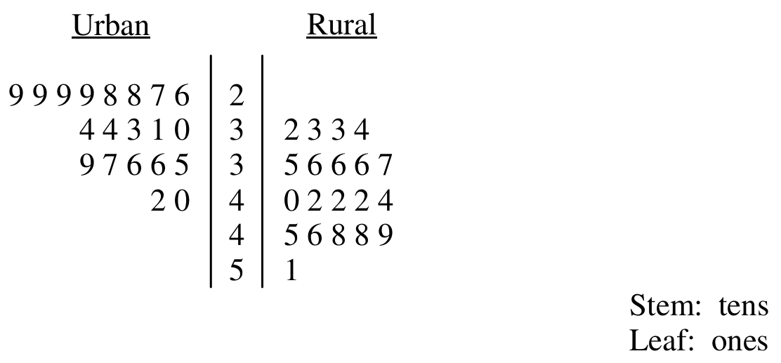
Reading the stemplot, the rural distribution is centered higher and is more spread out than the urban distribution.
For the rural students:
Mean \(\approx 40.45\) cal/kg
Median \(\approx 41\) cal/kg
Range \(= 19\)
SD \(\approx 6.04\)
IQR \(\approx 10\)
For the urban students:
Mean \(\approx 32.6\) cal/kg
Median \(\approx 32\) cal/kg
Range \(= 16\)
SD \(\approx 4.67\)
IQR \(\approx 7\)
So both the typical value and the spread are larger for the rural group. In terms of shape, the rural data look fairly symmetric and spread evenly between about 32 and 51 cal/kg, while the urban data appear skewed toward the larger values.
\( \boxed{\text{Rural: higher center and more spread; Urban: lower center, less spread, right-skewed}} \)
(b)
No. Each sample came from just one rural school and one urban school, so these two specific schools may not represent the much larger and more diverse population of all rural and urban ninth graders across the country. Because the schools themselves were not randomly chosen from all such schools, the results can’t be safely extended beyond these two schools.
\( \boxed{\text{No — only one school of each type was sampled, so results cannot be generalized nationally}} \)
(c)
Plan II is the better choice.
Both plans already adjust for body size by dividing calories by body weight, so that part is the same. The real issue is that a single day’s eating can be unusually high or low depending on what happened that day — a birthday party, a sick day, a weekend versus a school day, and so on. By recording food over a full 7-day period and averaging, Plan II smooths out this day-to-day variability and gives a more stable, precise picture of each student’s typical caloric intake.
\( \boxed{\text{Plan II — averaging over 7 days reduces day-to-day variability and gives a more precise estimate}} \)
Question
• Has a high school diploma
Most-appropriate topic codes (AP Statistics):
• Topic 3.3 — Constructing a Confidence Interval for a Population Proportion (Part \(\mathrm{b}\))
• Topic 1.11 — Random Sampling (Part \(\mathrm{c}\))
▶️ Answer/Explanation
(a)
One issue is that random-digit dialing only reaches people who have a telephone. People without a high school diploma tend to have lower-paying jobs, so they may be less likely to be able to afford phone service. As a result, this group could be underrepresented in the sample.
\( \boxed{\text{Households without phones are missed, and these are more likely to lack a diploma, so the estimate may be too low}} \)
(b)
The margin of error for a proportion is
\( ME=z^*\sqrt{\dfrac{p(1-p)}{n}} \)
We want \(ME=0.03\) with \(95\%\) confidence, so \(z^*=1.96\), and we use the pilot estimate \(p=0.22\):
\( 0.03=1.96\sqrt{\dfrac{0.22(0.78)}{n}} \)
Solving for \(n\), first isolate the square root:
\( \sqrt{\dfrac{0.22(0.78)}{n}}=\dfrac{0.03}{1.96} \)
Square both sides:
\( \dfrac{0.22(0.78)}{n}=\left(\dfrac{0.03}{1.96}\right)^2 \)
Solve for \(n\):
\( n=\dfrac{0.22(0.78)}{\left(\dfrac{0.03}{1.96}\right)^2} \)
\( n=\left(\dfrac{1.96}{0.03}\right)^2(0.22)(0.78) \)
\( n\approx 732.47 \)
Since \(n\) must be a whole number and we need at least this many respondents, we round up:
\( \boxed{n=733\text{ respondents}} \)
(c)
A good approach here is stratified random sampling, using each state as a stratum. Within every state, a random sample of adult heads of households would be selected and surveyed, with the sample size in each state chosen based on the precision needed for that state. Once all the state-level samples are collected, the results can be combined to produce an overall national estimate.
\( \boxed{\text{Stratified random sampling — treat each state as a stratum and take a random sample within each state}} \)
Question
Most-appropriate topic codes (AP Statistics):
• Topic 2.7 — Independent Events and Unions of Events (Part a,b)
• Topic 2.4 — Introduction to Probability (Part b)
• Topic 2.3 — Estimating Probabilities Using Simulation (Part c)
•Topic 1.12 — Potential Problems with Sampling (Part d)
▶️ Answer/Explanation
(a)
The probability distribution of \(X\) is not binomial because the bones are selected without replacement from a finite population of only 20 femurs. For a binomial distribution to apply, each trial must be independent — that is, the probability of success (selecting a male femur) must remain constant from one draw to the next. However, when sampling without replacement, the composition of the remaining pool changes with each selection, so the probability of drawing a male femur on each successive draw depends on what was drawn before it. Since the trials are not independent and the probability of success is not fixed, the distribution of \(X\) is hypergeometric, not binomial.
\(\boxed{X \text{ is not binomial because sampling is without replacement, making trials dependent}}\)
(b)
With 10 males and 10 females among the 20 brontosaurs, compute the probability that all 4 selected femurs are male using the multiplication rule for dependent events (without replacement):
\(P(\text{1st is male}) = \dfrac{10}{20}\)
\(P(\text{2nd is male} \mid \text{1st is male}) = \dfrac{9}{19}\)
\(P(\text{3rd is male} \mid \text{first two are male}) = \dfrac{8}{18}\)
\(P(\text{4th is male} \mid \text{first three are male}) = \dfrac{7}{17}\)
Therefore:
\(P(\text{all 4 are male}) = \dfrac{10}{20} \times \dfrac{9}{19} \times \dfrac{8}{18} \times \dfrac{7}{17}\)
\(= \dfrac{10 \times 9 \times 8 \times 7}{20 \times 19 \times 18 \times 17} = \dfrac{5040}{116280} \approx 0.0433\)
This can also be expressed using combinations:
\(P(\text{all 4 are male}) = \dfrac{\dbinom{10}{4}}{\dbinom{20}{4}} = \dfrac{210}{4845} \approx 0.0433\)
\(\boxed{P(\text{all 4 male}) \approx 0.0433}\)
(c)
No, it does not seem likely that males and females were equally represented in the group of 20 brontosaurs. From part (b), if the group had exactly 10 males and 10 females, the probability of randomly selecting 4 males in a row is only about \(4.33\%\). Since this probability is quite small (less than 5%), observing all 4 selected femurs being male is an unusual result under the assumption of equal representation. It is therefore more reasonable to think that males outnumbered females in this particular group of brontosaurs trapped in the swamp, though equal representation is possible — just unlikely given the data.
\(\boxed{\text{Equal representation is unlikely; evidence suggests more males than females in the group}}\)
(d)
No, it is not reasonable to generalize the conclusion from part (c) to the entire population of brontosaurs. The 20 brontosaurs found at the site do not constitute a random sample from the population of all brontosaurs — they represent only those individuals that happened to wander into that particular swamp and become trapped. This is a highly specific and non-random group. It is plausible that behavioral differences between male and female brontosaurs (for example, males may have been more likely to venture into deep swamp areas while foraging) could explain why males are overrepresented in this particular site. Such a non-representative sample cannot be used to draw conclusions about the broader population of all brontosaurs.
\(\boxed{\text{Cannot generalize; the 20 brontosaurs are not a random sample of all brontosaurs}}\)
Question
Many students believe that the food served in the dining hall needs improvement. Do you think that the quality of food served here needs improvement, even though that would increase the cost of the meal plan?
Most-appropriate topic codes (AP Statistics):
• Topic 1.12 — Potential Problems with Sampling (Parts a, b)
▶️ Answer/Explanation
(a)
Since the manager used a convenience sample — the first 100 students entering the cafeteria — bias may have been introduced because students who arrive at the dining hall early may have opinions about food quality that differ systematically from other dormitory residents who come later or not at all. For example, students who are very hungry or who have strong feelings about the food may be more likely to arrive early, making this group unrepresentative of all dormitory students.
To avoid this bias, the manager should have selected a random sample of 100 dormitory residents — for instance, using a simple random sample from a list of all dormitory residents, a stratified random sample by dormitory building, or a systematic random sample with a random starting point. Any of these approaches gives every dormitory resident a known, non-zero chance of being selected, which eliminates the selection bias introduced by the convenience sample.
(b)
The question as worded contains two sources of wording bias. First, the opening statement — “Many students believe that the food served in the dining hall needs improvement” — is leading because it tells respondents what other students think, which may pressure them to agree and respond “Yes” even if they do not truly feel that way.
Second, the phrase “even though that would increase the cost of the meal plan” introduces a second bias in the opposite direction, making students less likely to say “Yes” because they are reminded of a financial consequence. These two biases may push responses in opposite directions, making the results unreliable in either direction.
A better, more neutral wording would simply ask: “Do you think that the quality of food served in the dining hall needs improvement?” This removes the leading statement and the cost reminder, allowing students to respond based only on their true opinion about food quality.
Question
Most-appropriate topic codes (AP Statistics):
• Topic 3.13 — Carrying Out a Test for the Difference Between Two Population Proportions (Part a)
• Topic 3.1 — Estimators (Part b)
• Topic 1.11 — Random Sampling (Part c)
• Topic 1.12 — Potential Problems with Sampling (Part c)
▶️ Answer/Explanation
(a)
Step 1: State hypotheses.
Let \(p_A\) = true proportion of banded birds on Island A, and \(p_B\) = true proportion of banded birds on Island B.
\(H_0: p_A – p_B = 0 \qquad H_a: p_A – p_B \neq 0\)
Step 2: Identify the test and check assumptions.
We use a two-sample \(z\)-test for a difference in proportions. The test statistic is:
\(z = \dfrac{\hat{p}_A – \hat{p}_B}{\sqrt{\hat{p}(1-\hat{p})\left(\dfrac{1}{n_1} + \dfrac{1}{n_2}\right)}}\)
The problem states the samples are random. Since the two islands are separate, the samples are independent. We check the large sample condition using the pooled estimate:
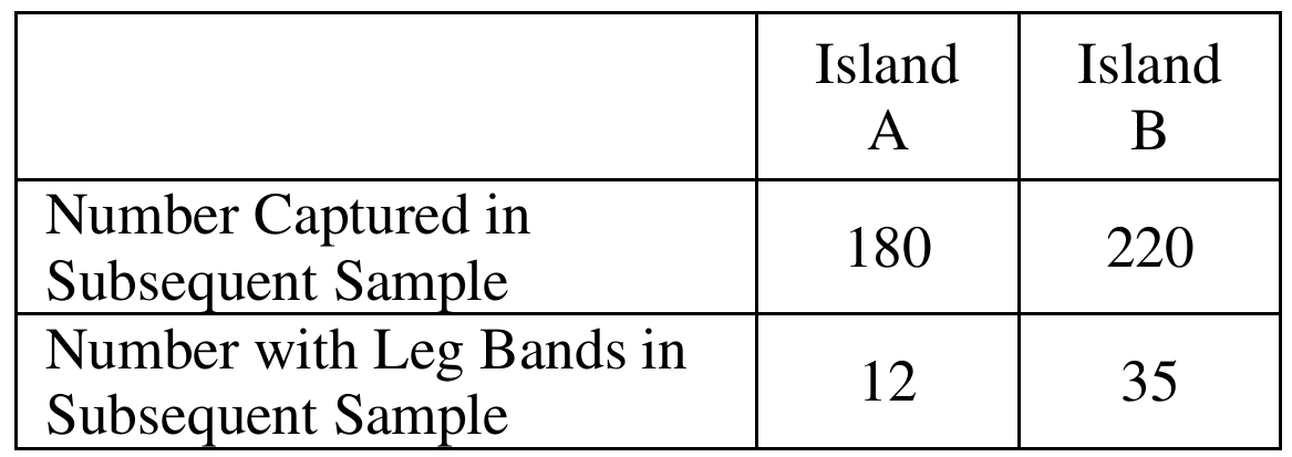
\(\hat{p} = \dfrac{n_A\hat{p}_A + n_B\hat{p}_B}{n_A + n_B} = \dfrac{12 + 35}{180 + 220} = \dfrac{47}{400} = 0.1175\)
Expected counts: \(n_A\hat{p} = 21.15,\quad n_A(1-\hat{p}) = 158.85,\quad n_B\hat{p} = 25.85,\quad n_B(1-\hat{p}) = 194.15\)
All expected counts are well above 5, so the large sample condition is satisfied.
Step 3: Compute the test statistic and p-value.
\(\hat{p}_A = \dfrac{12}{180} = 0.067 \qquad \hat{p}_B = \dfrac{35}{220} = 0.159\)
\(z = \dfrac{0.067 – 0.159}{\sqrt{\dfrac{(0.1175)(0.8825)}{180} + \dfrac{(0.1175)(0.8825)}{220}}} = \dfrac{-0.092}{\sqrt{0.00105}} = \dfrac{-0.092}{0.032} = -2.875\)
\(\text{p-value} = 2 \times P(Z < -2.875) \approx 0.00429\)
Step 4: State conclusion in context.
Since the p-value of \(0.00429\) is less than \(\alpha = 0.05\), we reject the null hypothesis. There is convincing statistical evidence that the proportions of banded birds on the two islands are different — Island B has a notably higher proportion of banded birds than Island A.
(b)
We use the capture-recapture logic: the proportion of banded birds in the subsequent sample estimates the proportion of banded birds in the whole population.
For Island A, the number of birds banded in the initial sample is \(n_I = 200\), and the proportion of banded birds observed in the subsequent sample is:
\(\hat{p}_S = \dfrac{12}{180} \approx 0.06667\)
Setting this equal to the fraction of banded birds in the population:
\(\hat{p}_S \approx \dfrac{n_I}{\text{population size}}\)
Solving for the estimated population size:
\(\text{Estimated population size} = \dfrac{n_I}{\hat{p}_S} = \dfrac{200}{12/180} = \dfrac{200 \times 180}{12} = \dfrac{36{,}000}{12} = \boxed{3{,}000 \text{ birds}}\)
(c)
Two concerns that should be addressed before assuming the captures can be treated as random samples are:
Concern 1 — Differential catchability: Some birds may be more likely to be captured than others — for example, slower, older, or less wary birds might be caught at a higher rate than the general population. If the same birds that were easy to capture in the initial sample are also more likely to appear in the subsequent sample, then banded birds would be overrepresented in the subsequent sample, leading us to underestimate the true population size.
Concern 2 — Behavioural change after banding: Birds that were captured and banded in the initial sample may become more trap-shy (avoiding capture in the future) or, conversely, may be more conspicuous to predators due to the bands, altering their survival or behaviour. If banded birds are less likely to be recaptured, we would overestimate the population size. In either case, if banding changes the birds’ behaviour or survival, the subsequent sample can no longer be treated as a true random sample of the population.
Question
Most-appropriate topic codes (AP Statistics):
• Topic 1.11 — Random Sampling (Part c)
• Topic 1.12 — Potential Problems with Sampling (Part c)
▶️ Answer/Explanation
(a)
If volunteers who work together are all placed in the same program, there’s a risk that something specific to their workplace situation gets mixed up with the effect of the program itself. For example, suppose this group’s department recently had a deadline pushed back, which on its own would lower everyone’s stress level in that department regardless of which program they’re doing. If this entire group ends up in, say, the tai chi group, then the drop in stress they experience could mistakenly be credited to tai chi, when really it was caused by the lighter workload.
Random assignment fixes this issue. By randomly assigning volunteers to the two programs instead of letting groups choose, we spread people from this department across both the tai chi and yoga groups. This way, any unusual circumstance affecting that department’s stress levels — like the deadline change — gets “evened out” between the two treatment groups rather than being concentrated in just one. Randomization helps make sure the two groups are comparable at the start, so that any difference we see at the end can be attributed to the program rather than to some other confounding factor.
(b)
Yes, a control group would add useful information. Without one, the company could only compare tai chi to yoga directly — they could say which of the two programs led to a bigger drop in stress, but they couldn’t say whether either program actually caused a reduction in stress at all.
Here’s the issue: stress levels might naturally go down over a \(10\)-week period for reasons that have nothing to do with either program — for instance, if the overall work environment becomes less hectic during that time, everyone’s stress might drop a little just from that. A control group, which doesn’t participate in either program but still has its stress measured at the start and end of the \(10\) weeks, gives a baseline for what “no treatment” looks like under those same conditions.
By comparing each treatment group’s change in stress to the control group’s change, the company can tell how much of the reduction is actually attributable to tai chi or yoga specifically, rather than just background changes that would have happened anyway.
(c)
No, it is not reasonable to generalize these findings to all employees of the company. The participants in this study were volunteers, not a random sample of employees. People who choose to volunteer for a stress-reduction study might already be different from the typical employee — for example, they might be more motivated to manage their stress, more open to trying tai chi or yoga, or have more flexible schedules that let them give up part of their lunch hour.
Because the group wasn’t randomly selected from the entire employee population, there’s no guarantee that what works (or doesn’t work) for these volunteers would apply the same way to employees who didn’t volunteer. So while the random assignment within the study supports drawing cause-and-effect conclusions about tai chi versus yoga for people like these volunteers, it doesn’t justify extending those conclusions to the company as a whole.