
AP Statistics 1.13 Experimental Design- Exam Style Questions - FRQs - New Syllabus
Question
Most-appropriate topic codes (AP Statistics):
• Topic \(1.13\) — Experimental Design (Part \( \mathrm{b} \))
▶️ Answer/Explanation
(a)
This is an observational study.
The researchers are simply gathering data by asking car owners to estimate their mileage, without actively imposing any treatments or randomly assigning participants to drive specific car models.
(b)
First, number the \(70\) days from \(1\) to \(70\).
Write the numbers \(1\) through \(70\) on identical slips of paper, place them into a hat, and mix them thoroughly.
Draw \(35\) slips of paper one by one without replacement.
The \(35\) days corresponding to the drawn numbers will be assigned the treatment of driving with the autopilot feature, and the remaining \(35\) days will be assigned to drive without the autopilot feature.
(c)
In order to generalize his findings to all Model D cars in his club, James cannot solely rely on an experiment conducted using only his own vehicle.
He would need to select a random sample of Model D cars (and their respective drivers) from the club’s membership to participate in his study.
Question
• Treatments
• Response variable
Most-appropriate topic codes (AP Statistics):
• Topic \(1.13\) — Experimental Design (Parts \( \mathrm{b} \), \( \mathrm{c} \))
▶️ Answer/Explanation
(a)
Experimental units: The 60 driveways (or the 60 new homes).
Treatments: The two types of concrete (concrete containing fibers and concrete without fibers).
Response variable: The severity of cracks in each driveway, measured on a scale of 0 to 10.
(b)
Number the 60 driveways from 1 to 60. Write the numbers 1 through 60 on identical slips of paper, place them in a hat, and mix thoroughly. Without looking, select 30 slips of paper one by one without replacement. The 30 driveways corresponding to the selected numbers will receive the concrete containing fibers, and the remaining 30 driveways will receive the concrete without fibers.
(c)
The primary benefit of random assignment is that it creates two treatment groups that are roughly equivalent at the beginning of the experiment. This helps to balance out the effects of potentially confounding variables, such as soil quality, driveway slope, or vehicle weight, across both groups. Because these other variables are distributed somewhat equally, the developer can confidently conclude that the statistically significant reduction in crack severity was actually caused by the addition of fibers to the concrete.
Question
• Experimental units:
• Response variable:
Most-appropriate topic codes (AP Statistics):
• Topic \(1.13\) — Experimental Design (Parts \( \mathrm{b} \), \( \mathrm{c} \))
▶️ Answer/Explanation
(a)
• Treatments: The new drug and the placebo.
• Experimental units: The 72 individual people (the 36 pairs of identical twins) participating in the experiment.
• Response variable: The improvement in acne severity, measured on a scale from 0 to 100.
(b)
A matched-pairs design controls for the variation in baseline acne severity and genetic/environmental factors among the subjects. Because identical twins share these traits, the difference in their acne improvement can be more directly attributed to the respective treatments rather than individual skin differences. This reduces the variability in the response and increases the statistical power to detect a true difference in effectiveness between the new drug and the placebo.
(c)
For each pair of identical twins, flip a fair coin. If the coin lands on heads, assign Twin A to receive the new drug and Twin B to receive the placebo. If the coin lands on tails, assign Twin A to receive the placebo and Twin B to receive the new drug. Repeat this random assignment process independently for all 36 pairs of twins.
Question
Most-appropriate topic codes (AP Statistics):
• Topic \(1.13\) — Experimental Design (Part \( \mathrm{c} \))
▶️ Answer/Explanation
(a)
Treatments: The four different concentrations of the fungus spray (\(0\,\text{ml/L}\), \(1.25\,\text{ml/L}\), \(2.5\,\text{ml/L}\), and \(3.75\,\text{ml/L}\)).
Experimental units: The \(20\) individual containers, each containing an equal number of insects.
Response variable: The number of insects that are still alive in each container one week after being sprayed.
(b)
Yes, the experiment definitely has a control group.
The containers sprayed with the \(0\,\text{ml/L}\) concentration form the control group because this specific mixture contains absolutely no fungus, serving as a baseline for comparison.
(c)
First, label each of the \(20\) containers with a unique integer from \(1\) to \(20\).
Next, use a random number generator to select \(15\) unique integers from \(1\) to \(20\) without replacement.
Assign the first five containers selected to receive the \(0\,\text{ml/L}\) treatment.
Assign the next five containers selected to receive the \(1.25\,\text{ml/L}\) treatment, and the next five to receive the \(2.5\,\text{ml/L}\) treatment.
Finally, the remaining five containers that were not selected will automatically receive the \(3.75\,\text{ml/L}\) treatment.
Question

Most-appropriate topic codes (AP Statistics):
• Topic \(4.5\) — Carrying Out a Test for a Difference of Two Population Means (Part \( \mathrm{b} \))
▶️ Answer/Explanation
(a)
Yes, because the study used random assignment to assign participants to the two treatment groups.
Detailed Solution:
Random assignment creates comparable groups by balancing out potential confounding variables between the standard and new procedure groups.
Because of this design, a statistically significant difference in mean recovery times can indeed be attributed to the causal effect of the surgery type.
The inference applies to the population of patients similar to those who participated in the study.
(b)
Yes, the data provide convincing evidence that the new procedure results in lower average recovery time.
Detailed Solution:
We perform a two-sample $t$-test for a difference in means ($\mu_{standard} – \mu_{new} > 0$).
Calculating the standard error: $SE = \sqrt{\frac{34^2}{110} + \frac{29^2}{100}} = \sqrt{10.509 + 8.41} \approx 4.35$.
Calculating the $t$-statistic: $t = \frac{(217 – 186) – 0}{4.35} \approx 7.13$.
With a $t$-score of approximately $7.13$, the $p$-value is extremely small (virtually $0$), which is less than any standard significance level like $\alpha = 0.05$.
Therefore, we reject the null hypothesis and conclude there is overwhelming statistical evidence that the new procedure reduces recovery time.
Question
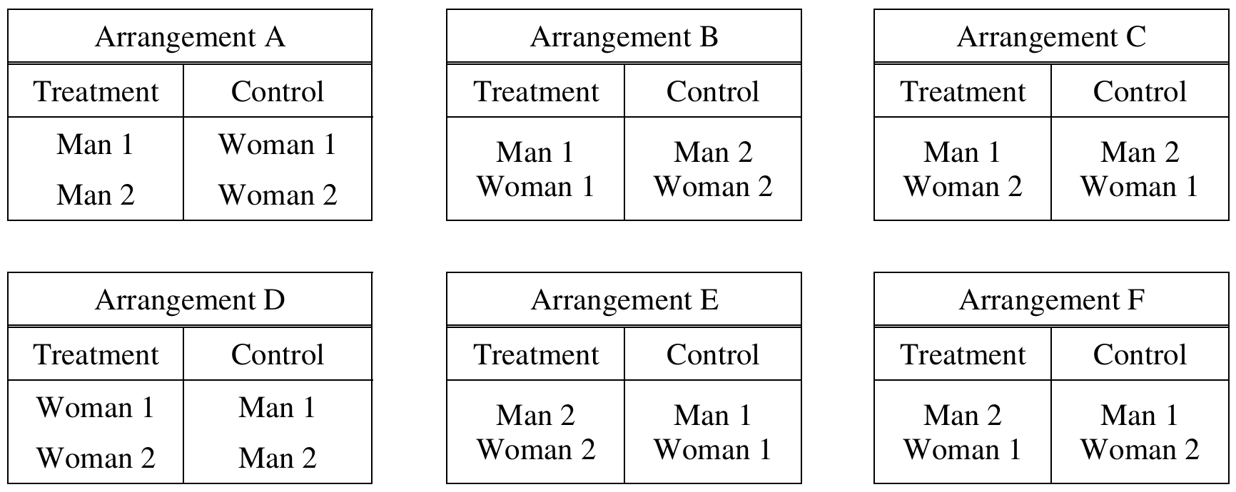
(i) Complete the table below by calculating the probability of each arrangement occurring if the sequential coin flip method is used.

(i) Complete the table below by calculating the probability of each arrangement occurring if the chip method is used.
Most-appropriate topic codes (AP Statistics):
• Topic \(2.6\) — Conditional Probability (Parts \( \mathrm{a} \), \( \mathrm{b} \))
• Topic \(2.7\) — Independent Events and Mutually Exclusive Events (Parts \( \mathrm{a} \), \( \mathrm{b} \))
▶️ Answer/Explanation
(a)(i)
Let T (tail) represent being assigned to the treatment group and H (head) represent being assigned to the control group. The process stops as soon as one group fills up. We trace each possible sequence of flips:

(a)(ii)
Man 1 and Man 2 are assigned to the same group only in Arrangements A (both in treatment) and D (both in control). So the probability is:
\(P(A) + P(D) = \dfrac{1}{4} + \dfrac{1}{4} = \boxed{\dfrac{1}{2}}\)
(b)(i)
Let T represent being assigned to the treatment group and C represent being assigned to the control group. Since chips are drawn without replacement from a pool of 2 T chips and 2 C chips, the probabilities change at each draw. Working through each arrangement:

(b)(ii)
Man 1 and Man 2 are in the same group only in Arrangements A and D. Therefore:
\(P(A) + P(D) = \dfrac{1}{6} + \dfrac{1}{6} = \boxed{\dfrac{1}{3}}\)
(c)
The chip method should be used. Here is the reasoning:
From parts (a)(i) and (b)(i), the chip method gives every arrangement an equal probability of \(\dfrac{1}{6}\), while the coin flip method assigns unequal probabilities — arrangements A and D each have probability \(\dfrac{1}{4}\), while B, C, E, and F each have probability \(\dfrac{1}{8}\).
From parts (a)(ii) and (b)(ii), the probability that both men end up in the same group is \(\dfrac{1}{2}\) under the coin method but only \(\dfrac{1}{3}\) under the chip method. Since students enter first and teachers enter next, the coin flip method is more likely to place all students together in one group — if teachers and students have different food preferences, this imbalance would make it impossible to tell whether any observed difference in lunch preference is due to the treatment (type of lunch) or the role of the participant (teacher vs. student).
The chip method, by giving all arrangements an equal chance, is therefore more appropriate for this experiment.
Question
Most-appropriate topic codes (AP Statistics):
• Topic \(3.14\) — Setting Up a Chi-Square Test for Homogeneity or Independence (Part \( \mathrm{a} \))
• Topic \(3.15\) — Carrying Out a Chi-Square Test for Homogeneity or Independence (Part \( \mathrm{a} \))
▶️ Answer/Explanation
(a)
Step 1: State hypotheses.
\(H_0\): There is no association between the type of ad viewed and children’s choice of snack (the proportion choosing each snack is the same regardless of which ad is viewed).
\(H_a\): There is an association between the type of ad viewed and children’s choice of snack (the proportions differ based on which ad is viewed).
Step 2: Identify the procedure and check conditions.
The appropriate procedure is a chi-square test of homogeneity (also acceptable: chi-square test of independence).
Conditions:
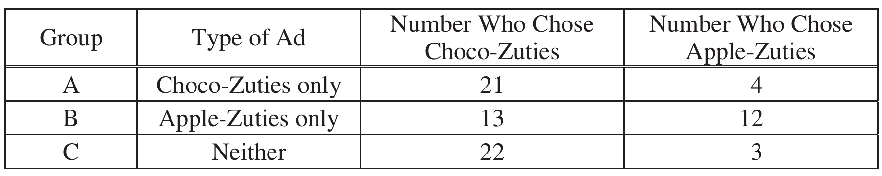
1. Random: The 75 children were randomly assigned to the three groups — this condition is satisfied.
2. Large Counts: All expected cell counts must be at least 5. The expected counts are computed as:
\( E = \frac{(\text{row total}) \times (\text{column total})}{\text{table total}} \)
Expected counts table (observed counts with expected counts in parentheses):

The smallest expected count is \(6.33 \geq 5\), so the large counts condition is satisfied. Both conditions are met.
Step 3: Calculate the test statistic and \(p\)-value.
The chi-square test statistic is:
\( \chi^2 = \sum \frac{(O – E)^2}{E} \)
\( \chi^2 \approx \frac{(21-18.67)^2}{18.67} + \frac{(4-6.33)^2}{6.33} + \frac{(13-18.67)^2}{18.67} + \frac{(12-6.33)^2}{6.33} + \frac{(22-18.67)^2}{18.67} + \frac{(3-6.33)^2}{6.33} \)
\( \chi^2 \approx 0.292 + 0.860 + 1.720 + 5.070 + 0.595 + 1.754 \approx 10.291 \)
Degrees of freedom: \(df = (r-1)(c-1) = (3-1)(2-1) = 2\)
The \(p\)-value: \(P\!\left(\chi^2_{\,df=2} \geq 10.291\right) \approx 0.006\)
Step 4: State a conclusion in context.
Because the \(p\)-value \(\approx 0.006\) is much smaller than \(\alpha = 0.05\), we reject \(H_0\). The data provide convincing statistical evidence that there is an association between the type of ad viewed and children’s choice of snack, among all children similar to those who participated in the experiment.
(b)
When neither ad was shown (Group C), \(\dfrac{22}{25} = 88\%\) of the children chose Choco-Zuties, and only 12% chose Apple-Zuties — this reflects the baseline preference without any advertising.
When children saw the Choco-Zuties ad (Group A), 84% still chose Choco-Zuties, which is very close to the 88% in the no-ad group. So the Choco-Zuties ad had very little effect on children’s snack choice — they were already inclined toward the sugary option anyway.
When children saw the Apple-Zuties ad (Group B), only \(\dfrac{13}{25} = 52\%\) chose Choco-Zuties, and 48% chose Apple-Zuties. This is a large shift compared to the 12% who chose Apple-Zuties in the no-ad group, meaning the Apple-Zuties ad had a substantial effect in increasing children’s likelihood of choosing the healthy snack.
Question
\(H_a : p_m – p_c < 0,\)
Most-appropriate topic codes (AP Statistics):
• Topic \(3.12\) — Setting Up a Test for the Difference Between Two Population Proportions (Part \( \mathrm{b} \))
• Topic \(3.13\) — Carrying Out a Test for the Difference Between Two Population Proportions (Part \( \mathrm{c} \))
• Topic \(2.3\) — Estimating Probabilities Using Simulation (Part \( \mathrm{c} \))
▶️ Answer/Explanation
(a)
No, it would not be reasonable to conclude that daily meditation causes a reduction in blood pressure. This study is an observational study — the men themselves chose whether or not to meditate; no treatment was randomly assigned. Because there was no randomization of treatment, cause-and-effect conclusions cannot be drawn from the results. Men who choose to meditate may differ from men who don’t in other important ways that are also related to blood pressure, such as being more health-conscious, exercising more, or having lower stress in general. These potential confounding variables make it impossible to isolate meditation as the cause.
(b)
For a normal approximation to be valid for the sampling distribution of \(\hat{p}_m – \hat{p}_c\), we need the number of successes and failures in each group to each be at least \(10\). First, compute the combined sample proportion of successes:
$\hat{p} = \frac{0 + 8}{11 + 17} = \frac{8}{28} \approx 0.286$
Then check each group:
For the meditation group \((n_m = 11)\):
$n_m \hat{p} = 11 \times \frac{8}{28} \approx 3.14 < 10 \quad \text{(condition fails)}$
For the non-meditation group \((n_c = 17)\):
$n_c \hat{p} = 17 \times \frac{8}{28} \approx 4.86 < 10 \quad \text{(condition fails)}$
Since the expected number of successes in both groups is less than \(10\), the normal approximation condition is not met, and it is not reasonable to use a normal approximation for the sampling distribution of \(\hat{p}_m – \hat{p}_c\).
(c)
First, compute the observed value of the sample statistic from the data:
$\hat{p}_m – \hat{p}_c = \frac{0}{11} – \frac{8}{17} \approx -0.47$
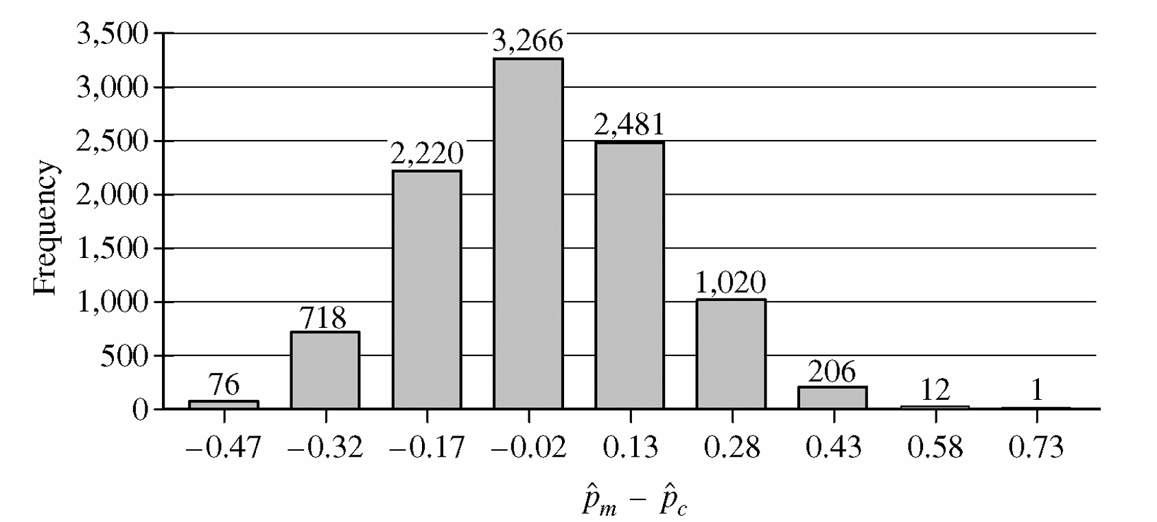
From the simulation histogram, only \(76\) out of \(10{,}000\) simulated values were \(-0.47\) or less (the most extreme negative outcome), giving an approximate \(p\)-value of:
$p\text{-value} \approx \frac{76}{10{,}000} = 0.0076$
Since this \(p\)-value of \(0.0076\) is very small (less than any common significance level such as \(\alpha = 0.05\)), we reject \(H_0\). There is convincing statistical evidence that men in this retirement community who meditate daily have a lower rate of high blood pressure than men who do not meditate. However, because this is an observational study, we can only conclude that meditation is associated with lower blood pressure — we cannot conclude that meditation causes a reduction in blood pressure.
Question
Most-appropriate topic codes (AP Statistics):
• Topic 1.13 — Experimental Design (Part b)
• Topic 1.13 — Experimental Design (Part c)
▶️ Answer/Explanation
(a)
This study was an experiment.
An experiment is defined by the active imposition of treatments on subjects by the researchers. In this case, the researchers randomly assigned the 27 participants to receive either the active treatment (the D-cycloserine pill) or the control treatment (the placebo).
If it were an observational study, the researchers would have merely observed pre-existing behaviors or treatment choices without intervening or assigning treatments.
(b)
No, the researchers would not be justified in drawing that conclusion.
The experiment only compared two treatment groups: two therapy sessions with D-cycloserine and two therapy sessions with a placebo. There was no treatment group in the study that received eight therapy sessions without the pill.
Because the study did not include a group receiving eight therapy sessions, it is impossible to make a direct, statistically valid comparison between the D-cycloserine + two sessions group and the standard eight sessions approach based solely on this study’s data.
(c)
Allowing therapists to choose the treatment assignments instead of using random assignment introduces selection bias and confounding variables.
If therapists are allowed to choose, they might assign the active D-cycloserine pill to patients they believe need it most (e.g., patients with more severe acrophobia) or to those they feel are most likely to respond positively. Conversely, they might assign the placebo to less severe cases.
This means the two groups would no longer be comparable at the start of the study. If a difference in improvement is observed at the end of the study, it would be impossible to determine whether the difference was caused by the D-cycloserine pill or by the initial, systematic differences in the severity of the patients’ acrophobia (the confounding variable).
Question
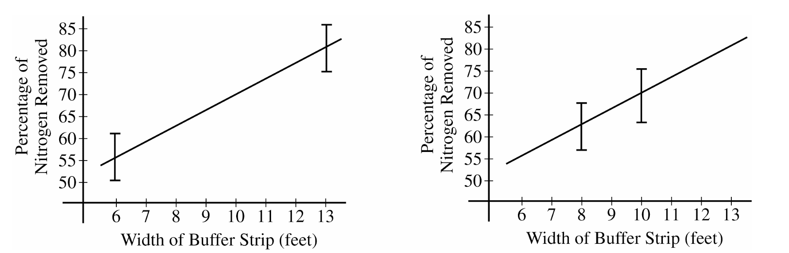
Most-appropriate topic codes (AP Statistics):
• Topic 4.1 — Sampling Distributions for Sample Means (Parts c, d)
• Topic 5.5 — Least-Squares Regression (Part e)
• Topic 1.13 — Experimental Design (Part f)
▶️ Answer/Explanation
(a)
(b)
(c)
(d)
(e)
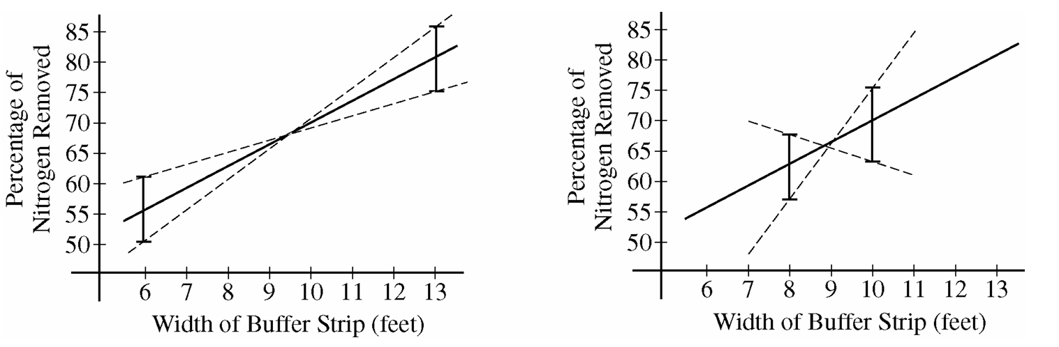
(f)
Question
ii. the experimental units
iii. the response that will be measured

ii. Based on your graph, do you think a linear regression model is appropriate? Explain.
Most-appropriate topic codes (AP Statistics):
• Topic 5.1 — Graphical Representations Between Two Quantitative Variables (Part b.i)
• Topic 5.3 — Linear Regression Models (Part b.ii)
▶️ Answer/Explanation
(a)
i. The treatments: The five different concentrations of garlic oil infused into the food granules, which are 0%, 2%, 10%, 25%, and 50%.
ii. The experimental units: The 40 individual European starlings (or the individual cages housing each bird).
iii. The response that will be measured: The number of food granules consumed by an individual bird during the two-hour period.
(b)
i. Graph construction:
To investigate linearity, we construct a scatterplot with Garlic Oil Concentration (%) on the horizontal $x$-axis and Mean Number of Food Granules Consumed on the vertical $y$-axis.
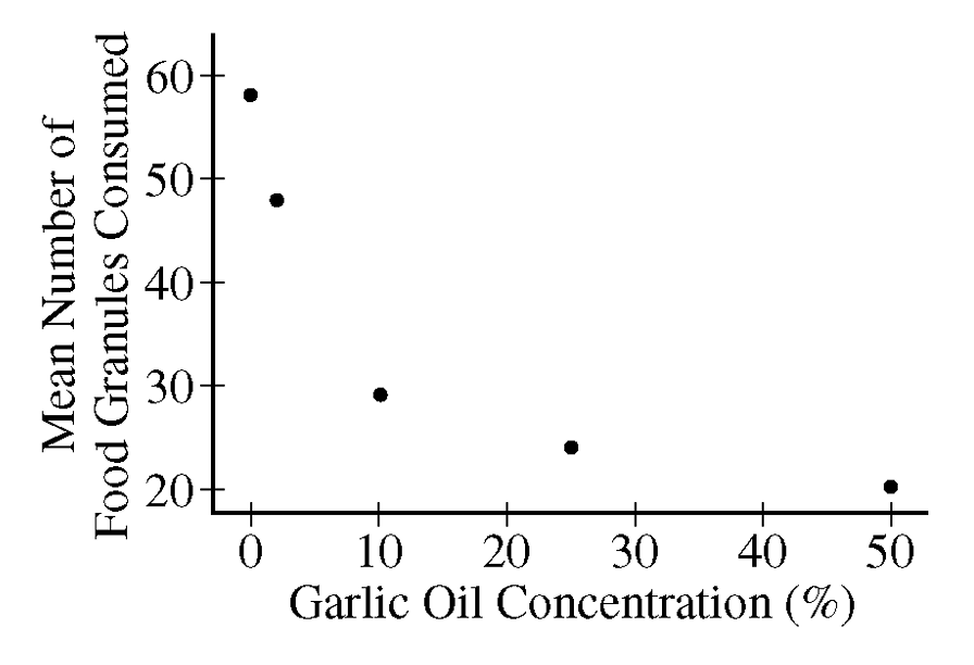
The points to plot are $(0, 58)$, $(2, 48)$, $(10, 29)$, $(25, 24)$, and $(50, 20)$.
ii. Linearity Assessment:
No, a linear regression model is not appropriate.
The scatterplot reveals a clear, distinct curved pattern rather than a straight line trend.
As the garlic oil concentration increases, the mean number of food granules consumed drops sharply at first and then begins to level off, indicating a non-linear relationship.
Question
Most-appropriate topic codes (AP Statistics):
• Topic \(1.13\) — Experimental Design (Part \(\mathrm{b}\))
• Topic \(1.12\) — Potential Problems with Sampling (Part \(\mathrm{b}\))
▶️ Answer/Explanation
(a) — Completely Randomized Design
Assign each of the 24 students a unique two-digit number from \(01\) to \(24\).
Use a random number table or a random number generator to produce a sequence of two-digit numbers from \(01\) to \(24\), ignoring repeats and any numbers outside that range.
The first 12 distinct numbers that appear correspond to the students assigned to the physical dissection program; the remaining 12 students are assigned to the computer simulation program.
This ensures both groups are of equal size (\(n = 12\) each) and that assignment is governed entirely by chance, removing any systematic differences between the groups before the study begins.
Alternative: Randomized Block Design
Rank all 24 students from lowest to highest pretest score.
Form 12 blocks of 2 students each: Block 1 contains the two students with the lowest pretest scores, Block 2 the next two, and so on, with Block 12 containing the two students with the highest pretest scores.
Within each block, randomly assign one student to the physical dissection program and the other to the computer simulation program — for example, by flipping a fair coin or using a random number generator to decide which student in each pair gets which treatment.
This design controls for prior knowledge of frog anatomy (as measured by the pretest), making the comparison between treatments more precise.
(b)
When students self-select into groups, the two groups may differ systematically in ways that affect posttest performance — completely apart from which instructional method they received.
For example, suppose students who already know a great deal about frog anatomy tend to be the ones who choose the physical dissection program, because they are enthusiastic about frogs and eager to work with them hands-on. Since these students enter with higher prior knowledge, there is less room for them to improve between the pretest and the posttest, so their score changes (posttest \(-\) pretest) will tend to be smaller.
Meanwhile, the students who choose the computer simulation tend to know less about frog anatomy to begin with, so they have more room to improve, and their score changes will tend to be larger.
If the computer simulation group shows a larger average improvement, we cannot tell whether the simulation program itself is more effective or whether the difference simply reflects the fact that lower-knowledge students had more room to grow. The self-selection has introduced a confounding variable (prior knowledge of frog anatomy) that makes it impossible to isolate the effect of the instructional method alone.
Question
Most-appropriate topic codes (AP Statistics):
• Topic \(3.13\) — Carrying Out a Test for the Difference Between Two Population Proportions (Part \(\mathrm{b}\): test statistic, \(p\)-value, and conclusion)
• Topic \(3.9\) — Sampling Distributions for the Difference Between Sample Proportions (Part \(\mathrm{a}\): large counts condition for inference)
• Topic \(1.13\) — Experimental Design (Part \(\mathrm{a}\): random assignment of treatments)
▶️ Answer/Explanation
Let \(p_A\) = true proportion of patients who survive at least one year if treated with the cardiopump.
Let \(p_B\) = true proportion of patients who survive at least one year if treated with CPR.
(a)
The two conditions required for a two-sample \(z\)-test comparing proportions in an experiment are:
Condition 1 — Random assignment of treatments: Before the study began, a coin was tossed to determine which treatment was assigned to even-numbered days and which to odd-numbered days. This coin toss serves as a reasonable approximation to randomly assigning the two treatments to the available subjects, so this condition is satisfied.
Condition 2 — Sufficiently large sample sizes: All four counts (successes and failures for each group) must be at least 5. Checking:
\(n_A \hat{p}_A = 37 \geq 5, \quad n_A(1-\hat{p}_A) = 754 – 37 = 717 \geq 5\)
\(n_B \hat{p}_B = 15 \geq 5, \quad n_B(1-\hat{p}_B) = 746 – 15 = 731 \geq 5\)
All four values are well above 5, so the large sample condition is satisfied.
(b)
Step 1 — Hypotheses:
\(H_0: p_A = p_B \quad \text{(or } p_A – p_B = 0\text{)}\)
\(H_a: p_A > p_B \quad \text{(or } p_A – p_B > 0\text{)}\)
Step 2 — Test: Two-sample \(z\)-test for proportions (one-sided).
Step 3 — Compute the test statistic:
First, compute the pooled sample proportion:
\(\hat{p} = \frac{n_A \hat{p}_A + n_B \hat{p}_B}{n_A + n_B} = \frac{37 + 15}{754 + 746} = \frac{52}{1500} \approx 0.0347\)
Now compute the \(z\)-statistic:
\(z = \frac{\hat{p}_A – \hat{p}_B}{\sqrt{\hat{p}(1-\hat{p})\left(\dfrac{1}{n_A} + \dfrac{1}{n_B}\right)}}\)
\(z = \frac{\dfrac{37}{754} – \dfrac{15}{746}}{\sqrt{(0.0347)(1 – 0.0347)\left(\dfrac{1}{754} + \dfrac{1}{746}\right)}} \approx 3.066\)
The corresponding one-sided \(p\)-value is:
\(p\text{-value} = P(Z > 3.066) \approx 0.0011\)
Step 4 — Conclusion:
Since the \(p\)-value of \(0.0011\) is much less than any reasonable significance level (such as \(\alpha = 0.05\) or \(\alpha = 0.01\)), we reject \(H_0\).
There is strong statistical evidence that the proportion of patients who survive at least one year is higher when treated with the cardiopump than when treated with CPR — that is, the cardiopump has a significantly higher survival rate than CPR.
Question
Treatment 2: A blue background with narrow red stripes
Most-appropriate topic codes (AP Statistics):
• Topic \(1.13\) — Experimental Design (Part \(\mathrm{a}\): blocking on bird species to reduce variability)
• Topic \(4.8\) — Justifying a Claim Based on a Confidence Interval for the Difference Between Two Population Means (Part \(\mathrm{b}\): power and ability to detect treatment differences)
• Topic \(4.10\) — Carrying Out a Test for the Difference Between Two Population Means (Part \(\mathrm{b}\): factors affecting power, including sample size and significance level)
▶️ Answer/Explanation
(a)
Form three blocks based on species: Block 1 = blackbirds, Block 2 = starlings, Block 3 = geese. Since there are 100 birds of each species, each block contains 100 birds.
Within each block, randomly assign the 100 birds to the two treatments as follows:
Label each bird in the block with a unique number from 00 to 99. Use a random number table, calculator, or statistical software to generate a list of 50 distinct two-digit numbers between 00 and 99. The birds whose labels match these 50 numbers are assigned Treatment 1 (red background with narrow blue stripes). The remaining 50 birds in the block are assigned Treatment 2 (blue background with narrow red stripes).
Repeat this exact randomization procedure independently within Block 2 (starlings) and Block 3 (geese).
This results in 50 birds per treatment within each species block, and the random assignment ensures that any differences observed between treatments are not due to systematic differences among the birds.
(b)
One effective way to increase the power of the test (other than blocking) is to increase the sample size.
Increasing the number of birds in the study reduces the standard error of the sampling distribution of the difference in sample means.
A smaller standard error means the test statistic will be larger for any given true difference between treatments, making it more likely that the test will detect a real difference if one exists — that is, the power of the test increases.
Another valid approach is to increase the significance level \(\alpha\) (for example, from \(\alpha = 0.01\) to \(\alpha = 0.05\)). Raising \(\alpha\) makes it easier to reject a false null hypothesis, which lowers the probability of a Type II error (\(\beta\)), and since power \(= 1 – \beta\), the power increases.
Question
Most-appropriate topic codes (AP Statistics):
• Topic \(3.10\) — Constructing a Confidence Interval for the Difference Between Two Population Proportions (Part \(\mathrm{b}\))
• Topic \(3.11\) — Justifying a Claim Based on a Confidence Interval for the Difference Between Two Population Proportions (Parts \(\mathrm{b}\), \(\mathrm{e}\))
• Topic \(3.1\) — Estimators (Part \(\mathrm{c}\): estimating relative risk using \(\hat{p}_A/\hat{p}_B\))
• Topic \(3.11\) — Justifying a Claim Based on a Confidence Interval for the Difference Between Two Population Proportions (Part \(\mathrm{d}\): interpreting the confidence interval for relative risk)
▶️ Answer/Explanation
(a)
Yes, this experiment can be performed as a double-blind experiment by introducing placebos for each treatment group.
Patients assigned to treatment A (pill) would also receive a placebo injection. Patients assigned to treatment B (injection) would also receive a placebo pill. This way, every patient receives both a pill and an injection, but one of the two is a placebo.
Since neither the patients nor the physicians administering the treatments know which is the real treatment and which is the placebo, neither group is aware of the treatment assignment — making the experiment double-blind.
(b)
First, compute the sample proportions:
\(\hat{p}_A = \frac{38}{154} \approx 0.2468, \qquad \hat{p}_B = \frac{16}{164} \approx 0.0976\)
The 95% confidence interval for \(p_A – p_B\) is:
\(\hat{p}_A – \hat{p}_B) \pm z^* \sqrt{\frac{\hat{p}_A(1-\hat{p}_A)}{n_A} + \frac{\hat{p}_B(1-\hat{p}_B)}{n_B}}\)
\(0.2468 – 0.0976) \pm 1.96\sqrt{\frac{(0.2468)(0.7532)}{154} + \frac{(0.0976)(0.9024)}{164}}\)
\(0.1492 \pm 1.96(0.0418)\)
\(0.1492 \pm 0.0818\)
\(\boxed{(0.0674,\ 0.2310)}\)
We are 95% confident that the true difference in 15-year survival rates \((p_A – p_B)\) is between \(0.0674\) and \(0.2310\). Because the entire interval lies above zero, this provides evidence that treatment A has a higher 15-year survival rate than treatment B.
(c)
The estimated relative risk is:
\(\frac{\hat{p}_A}{\hat{p}_B} = \frac{38/154}{16/164} = \frac{0.2468}{0.0976} \approx 2.53\)
\(\boxed{\text{Estimated relative risk} \approx 2.53}\)
This means patients receiving treatment A are estimated to be about 2.53 times as likely to survive at least 15 years as patients receiving treatment B.
(d)
A 95% confidence interval for \(\ln\!\left(\dfrac{p_A}{p_B}\right)\) is given as \((0.3868,\ 1.4690)\).
To convert this to a confidence interval for the relative risk \(\dfrac{p_A}{p_B}\), apply the exponential (inverse of the natural log) to each endpoint:
\(e^{0.3868} \approx 1.47 \qquad \text{and} \qquad e^{1.4690} \approx 4.34\)
\(\boxed{\left(1.47,\ 4.34\right)}\)
We are 95% confident that patients receiving treatment A are between 1.47 and 4.34 times as likely to survive at least 15 years compared to patients receiving treatment B.
(e)
When the survival proportions are small (as here, approximately 0.25 and 0.10), the confidence interval for the relative risk is more informative and practically meaningful than the confidence interval for the difference in proportions.
Knowing that a patient’s chance of survival is between 1.47 and 4.34 times greater with treatment A is more vivid and easier to interpret clinically than knowing the absolute difference in proportions is somewhere between 0.07 and 0.23 — a range that may sound small even though it represents a substantial relative advantage.
Question
Most-appropriate topic codes (AP Statistics):
• Topic 4.4 — Setting Up a Test for a Population Mean or Population Mean Difference (Part \(\mathrm{b}\))
• Topic 3.8 — Potential Errors When Performing Tests (Part \(\mathrm{b}\))
▶️ Answer/Explanation
(a)
Proposed Design (Completely Randomized Design):
Assign each of the 100 patients a unique number from 00 to 99. Using a random number table (or random number generator), select 50 unique numbers. The patients corresponding to the selected numbers will form Group 1 (Music Treatment); the remaining 50 patients will form Group 2 (Control — Noise-Free Environment).
Measure the diastolic blood pressure of every patient before the treatment begins. Then:
Group 1 patients sit quietly in a room where soothing music is played for 20 minutes.
Group 2 patients sit quietly in a noise-free environment for 20 minutes.
At the end of the 20-minute period, measure the diastolic blood pressure of every patient again. Compute the reduction in diastolic blood pressure (before \(-\) after) for each patient. Run a two-sample \(t\)-test to compare the mean reduction in the two groups.
Alternatively (Paired Design):
Each patient receives both treatments on two separate occasions, with a suitable washout period in between. For each patient, flip a coin to randomly assign which treatment is administered first. Compute the difference (music reduction \(-\) noise-free reduction) for each patient, and use a paired \(t\)-test to determine whether the mean difference is significantly greater than zero.
(b)
Let \(\mu_M\) = mean reduction in diastolic blood pressure under the music treatment, and \(\mu_C\) = mean reduction under the control (noise-free) treatment. The hypotheses are:
\(H_0: \mu_M = \mu_C \qquad H_a: \mu_M > \mu_C\)
Type I Error:
Rejecting \(H_0\) when it is actually true — that is, concluding that soothing music does reduce diastolic blood pressure more than sitting quietly, when in reality it does not.
Consequence: The clinic will offer music therapy as a free service to its patients even though the therapy is ineffective. This wastes clinic resources and money, providing no real medical benefit to patients.
Type II Error:
Failing to reject \(H_0\) when it is actually false — that is, concluding that soothing music does not reduce diastolic blood pressure more than sitting quietly, when in reality it does.
Consequence: The clinic will not offer music therapy, even though the therapy would genuinely help patients reduce their blood pressure. Patients are denied access to an effective, low-cost treatment.
Which error is more serious?
A reasonable case can be made for either error. One well-supported argument is that the Type II error is more serious: denying patients an effective treatment that could meaningfully improve their health — and potentially save lives — is a greater harm than wasting some clinic resources on an ineffective service. In the case of a Type I error, patients who receive music therapy are unlikely to be harmed by listening to music. But in the case of a Type II error, patients who could benefit from a real treatment are denied it altogether.
Question
Most-appropriate topic codes (AP Statistics):
• Topic 1.10 — The Investigative Question Revisited and Data Collection (Part \(\mathrm{a}\))
• Topic 1.11 — Random Sampling (Part \(\mathrm{b}\))
▶️ Answer/Explanation
(a)
A control group gives the researchers a baseline comparison group — without any dietary supplement — so they can measure whether glucosamine or chondroitin actually makes a difference beyond what would happen due to the normal aging process alone.
Without a control group, we could not tell whether any improvements in joint and hip health were caused by the supplements or simply by other factors such as the passage of time, veterinary care, or natural variation between dogs.
In this study specifically, the control group allows us to isolate the true effect of glucosamine and chondroitin on reducing canine osteoarthritis by comparing both treatment groups against untreated dogs under the same conditions.
\(\boxed{\text{Control group provides a baseline to determine whether the supplements are truly effective.}}\)
(b)
First, assign each of the 300 dogs a unique number from \(001\) to \(300\).
Then, use a random number generator (calculator, statistical software, or a random number table) to randomly select 100 numbers from \(001\) to \(300\), ignoring any repeats — the dogs corresponding to these 100 numbers are assigned to the glucosamine group.
From the remaining 200 dogs, randomly select another 100 numbers using the same process — these dogs are assigned to the chondroitin group.
The final 100 remaining dogs are assigned to the control group and receive no dietary supplement.
\(\boxed{\text{Randomly assign dogs numbered } 001\text{–}300 \text{ into three equal groups of 100 using a random number generator.}}\)
(c)
The blocking variable should be the one that has a stronger association with the response variable — joint and hip health — so that dogs within each block are as similar (homogeneous) as possible.
Breed of dog is associated with the size of the dog, and size is known to be related to joint and hip health — larger breeds tend to have more joint problems than smaller breeds, so breed is likely to create more variability in the response.
Clinic, on the other hand, is less likely to be strongly associated with joint and hip health because most large veterinary practices see a wide variety of dog breeds and sizes, so dogs across clinics would not be meaningfully more similar to each other than dogs across breeds.
Therefore, we should block on breed of dog, since it is more strongly related to joint and hip health and will reduce variability more effectively within each block.
\(\boxed{\text{Block on breed of dog, as it has a stronger relationship to joint and hip health than clinic.}}\)
Question
Most-appropriate topic codes (AP Statistics):
• Topic 3.12 — Setting Up a Test for the Difference Between Two Population Proportions (Part \(\mathrm{b}\))
• Topic 3.13 — Carrying Out a Test for the Difference Between Two Population Proportions (Part \(\mathrm{c}\))
• Topic 3.6 — p-Values (Part \(\mathrm{d}\))
• Topic 3.13 — Carrying Out a Test for the Difference Between Two Population Proportions (Part \(\mathrm{d}\))
▶️ Answer/Explanation
(a)
This study is classified as an experiment, not an observational study.
The key reason is that the researchers actively imposed treatments on the subjects — they randomly assigned drivers to one of two conditions: driving while using a cell phone, or driving while talking to a passenger.
In an observational study, researchers simply observe subjects without intervening; here, the environment was deliberately controlled and manipulated, which is the defining feature of an experiment.
\(\boxed{\text{Experiment — treatments (cell phone vs. passenger) were actively imposed on randomly assigned subjects.}}\)
(b)
Let \(p_{\text{cell}}\) = the population proportion of drivers who miss the exit while talking on a cell phone.
Let \(p_{\text{pass}}\) = the population proportion of drivers who miss the exit while talking to a passenger.
\(H_0: p_{\text{cell}} = p_{\text{pass}}\) (no difference in the proportion of drivers who miss the exit between the two groups)
\(H_a: p_{\text{cell}} > p_{\text{pass}}\) (a greater proportion of cell phone users miss the exit compared to passenger talkers)
\(\boxed{H_0: p_{\text{cell}} = p_{\text{pass}}, \quad H_a: p_{\text{cell}} > p_{\text{pass}}}\)
(c)
The two conditions required for a two-sample \(z\)-test for proportions are:
Condition 1 — Independent random samples or random assignment: The problem states that the 48 participants were randomly assigned to the two groups, so this condition is met.
Condition 2 — Large sample sizes (each of \(n_1\hat{p}_1\), \(n_1(1-\hat{p}_1)\), \(n_2\hat{p}_2\), \(n_2(1-\hat{p}_2)\) must be \(\geq 10\)):
For the cell phone group: \(n_1\hat{p}_1 = 24\cdot\dfrac{7}{24} = 7 < 10\)
For the passenger group: \(n_2\hat{p}_2 = 24\cdot\dfrac{2}{24} = 2 < 10\)
Both groups fail the large sample condition, so this condition is not met. A two-sample \(z\)-test is therefore not appropriate for this situation.
\(\boxed{\text{Condition 1 met (random assignment); Condition 2 NOT met } (n\hat{p} < 10 \text{ for both groups).}}\)
(d)
In everyday language, the \(p\)-value of \(0.0683\) means: assuming that cell phone use and talking to a passenger are equally distracting (i.e., \(H_0\) is true), there is about a \(6.83\%\) chance of observing a difference in missed-exit proportions as large as or larger than what was seen in this study just by random chance alone.
Since the \(p\)-value of \(0.0683\) is greater than \(\alpha = 0.05\), we fail to reject \(H_0\). We do not have statistically significant evidence at the 5% level to conclude that drivers using a cell phone are more distracted (as measured by missing the freeway exit) than drivers talking to a passenger.
\(\boxed{p\text{-value} = 0.0683 > 0.05 \Rightarrow \text{Fail to reject } H_0; \text{ insufficient evidence that cell phone use causes more distraction.}}\)
Question
Most-appropriate topic codes (AP Statistics):
• Topic 1.13 — Experimental Design (Control of Variability in Experimental Units) (Part \(\mathrm{c}\))
• Topic 1.13 — Experimental Design (Scope of Inference and Generalizability) (Part \(\mathrm{d}\))
▶️ Answer/Explanation
(a)
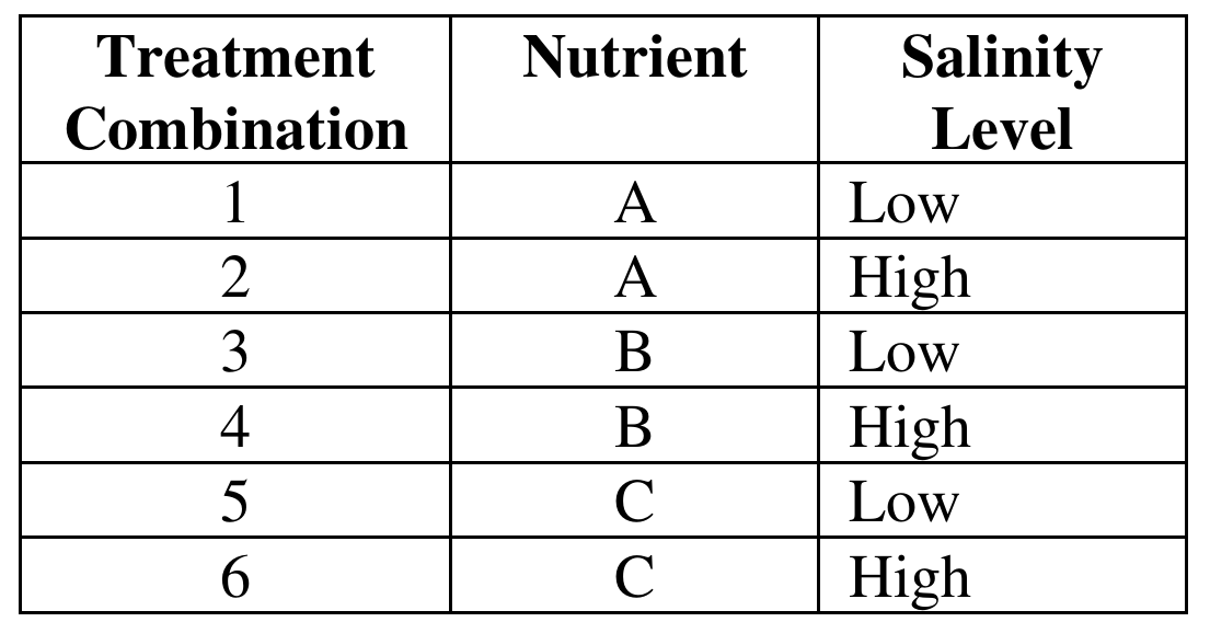
The biologist has 3 nutrients and 2 salinity levels, giving \(3 \times 2 = 6\) treatment combinations in total. The six treatments are:
(b)
Since 10 tiger shrimps have already been randomly placed into each of 12 similar tanks in a controlled environment, we must randomly assign the treatment combinations to the tanks. Each treatment combination will be randomly assigned to 2 of the 12 tanks. One way to do this is to generate a random number for each tank. The treatment combinations are then assigned by sorting the random numbers from smallest to largest.
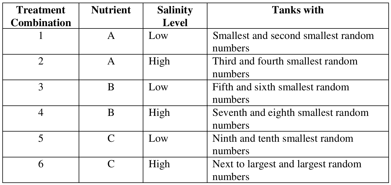
After three weeks, record the growth (weight gain = after \(-\) before) for the shrimps in each tank, and compare the average growth across tanks for each of the six treatment combinations.
(c)
Statistical advantage: Reduced variability among experimental units.
Tiger shrimps are more similar to one another in their natural growth characteristics than a mix of different shrimp species would be. By using only tiger shrimps, the biologist eliminates the shrimp species as a source of variation among the experimental units (the tanks). With less background variability in the response (growth), any real differences in growth due to the nutrient or salinity treatments are easier to detect — that is, the experiment has greater power to identify treatment effects that are actually present.
(d)
Statistical disadvantage: Limited scope of inference (reduced generalizability).
Because the experiment uses only tiger shrimps, the conclusions can only be applied to tiger shrimps. Other species of shrimp may respond differently to the same nutrient and salinity treatments, so the biologist cannot generalize the results to shrimps in general. The scope of inference is restricted solely to tiger shrimps, which limits the practical usefulness of the study if the biologist’s broader goal is to understand shrimp growth across species.
Question
Identify the treatments.
What were the experimental units?
Most-appropriate topic codes (AP Statistics):
• Topic 1.13 — Experimental Design (Part \(\mathrm{b}\): random assignment of treatments)
• Topic 1.13 — Experimental Design (Part \(\mathrm{c}\): replication)
• Topic 1.13 — Experimental Design (Part \(\mathrm{d}\): confounding variables)
▶️ Answer/Explanation
(a)
Response variable: The response variable is the amount of draft — that is, the energy required to pull the plow through the agricultural field.
Treatments: The two treatments are the standard hitch and the newly developed hitch.
Experimental units: The experimental units are the two large plots of land.
\(\boxed{\text{Response variable: draft} \quad \text{Treatments: standard hitch, new hitch} \quad \text{Experimental units: two plots of land}}\)
(b)
Yes, randomization was used properly in this study. It was randomly determined which of the two plots of land would be plowed using the standard hitch, meaning the two treatments (hitches) were randomly assigned to the two experimental units (plots). This random assignment helps reduce the potential for bias in comparing the two hitches, since neither hitch was systematically favored by being assigned to a particular plot.
\(\boxed{\text{Yes — treatments were randomly assigned to experimental units}}\)
(c)
No, replication was not used properly in this study. Each treatment (hitch type) was applied to only one experimental unit (plot of land). Replication requires that each treatment be applied to more than one experimental unit, so that general patterns can be observed and random variation can be distinguished from true treatment effects. Since each hitch was tested on only a single plot, there is no replication, and it is not possible to draw reliable conclusions about the draft-reducing capability of the new hitch from this study alone.
\(\boxed{\text{No — each hitch was applied to only one plot; proper replication requires multiple plots per treatment}}\)
(d)
Plot of land is a confounding variable because each hitch was used exclusively on one plot of land. The two plots may differ in environmental characteristics such as soil type, terrain, and moisture level, all of which can affect the draft. As a result, if a difference in draft is observed between the two hitches, it is impossible to determine whether that difference is due to the type of hitch or due to the inherent differences between the two plots. The effect of the hitch is therefore confounded with — that is, mixed up with — the effect of the plot of land.
\(\boxed{\text{Hitch effect cannot be separated from plot effect} \implies \text{plot of land is a confounding variable}}\)
Question
Most-appropriate topic codes (AP Statistics):
• Topic 3.2 — Sampling Distributions for Sample Proportions (Part \(\mathrm{b}\))
• Topic 2.10 — The Binomial Distribution (Part \(\mathrm{c}\))
• Topic 3.6 — p-Values (Part \(\mathrm{d}\))
• Topic 3.7 — Carrying Out a Test for a Population Proportion (Part \(\mathrm{e}\))
• Topic 1.13 — Experimental Design (Part \(\mathrm{f}\))
▶️ Answer/Explanation
(a)
Let \(p\) be the population proportion of consumers who prefer Citrus Fresh. The hypotheses are:
\(H_0: p = 0.5\)
\(H_a: p \neq 0.5\)
A two-sided alternative is appropriate because Sunshine Farms wants to detect any difference in preference, not just preference for one particular juice.
(b)
The conditions for a one-proportion \(z\)-test require that both \(np\) and \(n(1-p)\) be at least 5 (or 10). Here:
\(np = 8 \times 0.5 = 4 < 5\)
\(n(1-p) = 8 \times 0.5 = 4 < 5\)
Since both values are less than 5, the large-sample normal approximation is not valid, and using a one-proportion \(z\)-test would not be appropriate for a sample of only \(n = 8\).
(c)
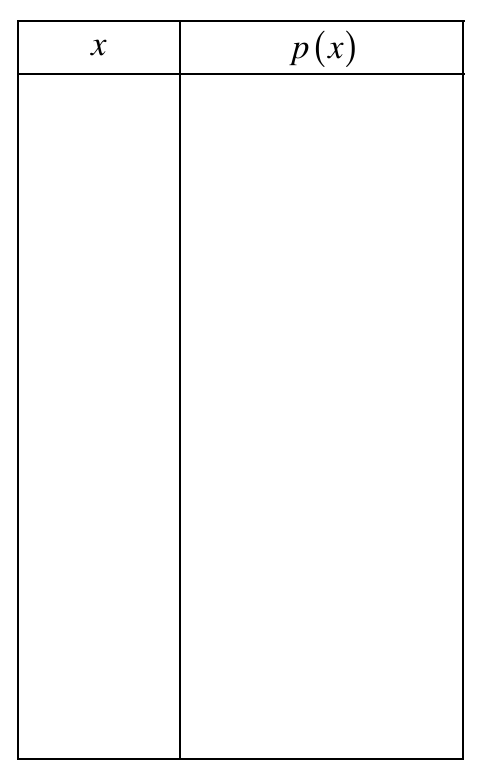
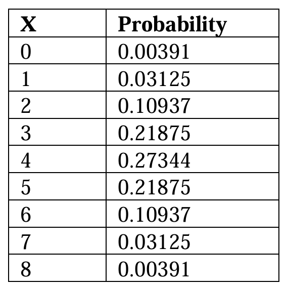
Under \(H_0\), \(X \sim \text{Binomial}(n = 8,\ p = 0.5)\). The probabilities are computed using:
\(P(X = x) = \binom{8}{x}(0.5)^x(0.5)^{8-x} = \binom{8}{x}(0.5)^8\)
(d)
No, it is not possible for the significance level to be exactly 0.05. Because \(X\) is a discrete random variable, the tail probabilities can only take specific values — there is no rejection region that gives a type I error probability of exactly 0.05.
The most extreme rejection region \((X = 0 \text{ or } X = 8)\) gives:
\(\alpha = 2 \times 0.00391 = 0.00782 < 0.05\)
The next possible rejection region \((X \leq 1 \text{ or } X \geq 7)\) gives:
\(\alpha = 2 \times (0.00391 + 0.03125) = 2 \times 0.03516 = 0.07031 > 0.05\)
Since no rejection region produces a type I error probability of exactly 0.05, a significance level of exactly 0.05 is not achievable with this test.
\(\boxed{\alpha = 0.05 \text{ is not achievable — the achievable levels jump from } 0.00782 \text{ to } 0.07031}\)
(e)
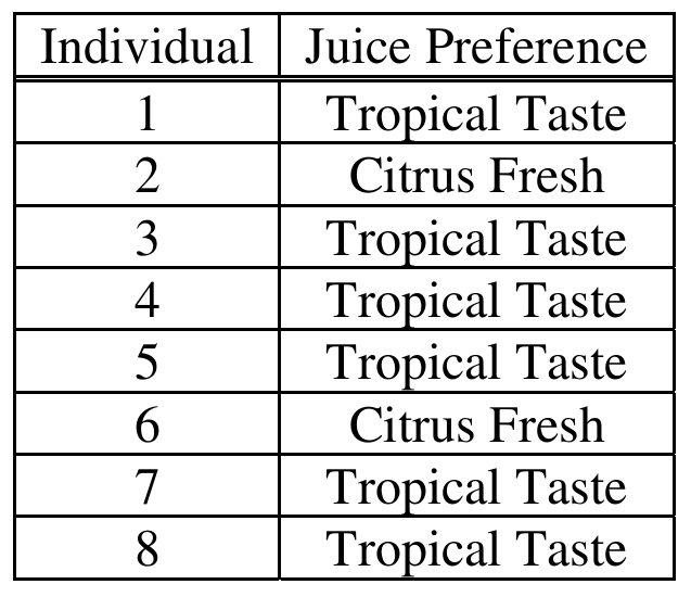
From the data, 2 out of 8 consumers preferred Citrus Fresh, so \(X = 2\).
Since this is a two-sided test, the \(p\)-value is the probability of observing a result at least as extreme as \(X = 2\) in either tail:
\(p\text{-value} = P(X \leq 2) + P(X \geq 6)\)
\(= 2 \times [P(X=0) + P(X=1) + P(X=2)]\)
\(= 2 \times (0.00391 + 0.03125 + 0.10937)\)
\(= 2 \times 0.14453 = 0.28906\)
Since the \(p\)-value of \(0.289\) is much larger than any reasonable significance level (e.g., \(\alpha = 0.05\) or \(\alpha = 0.07031\)), we fail to reject \(H_0\). There is not statistically significant evidence of a consumer preference between Citrus Fresh and Tropical Taste.
\(\boxed{p\text{-value} \approx 0.289 \implies \text{Fail to reject } H_0; \text{ no significant consumer preference detected}}\)
(f)
The most important recommendation is to increase the number of consumers in the study. With only \(n = 8\) consumers, the test has very low power — even a large true difference in preference (like 75% vs. 25%) may not produce a statistically significant result. Increasing the sample size would reduce the standard error of the estimated proportion \(\hat{p}\), making it easier to detect a real difference, and would allow the use of the large-sample one-proportion \(z\)-test since \(np \geq 5\) and \(n(1-p) \geq 5\) would be satisfied. For example, with \(n = 80\) and \(X = 20\) (same sample proportion of 0.25), the \(z\)-statistic would be approximately:
\(z = \frac{0.25 – 0.5}{\sqrt{\frac{0.5(0.5)}{80}}} \approx -4.47\)
which gives a \(p\)-value near zero, allowing a clear conclusion to be reached.
\(\boxed{\text{Recommendation: Increase sample size to increase power and enable use of the } z\text{-test}}\)
Question
Most-appropriate topic codes (AP Statistics):
• Topic 4.4 — Setting Up a Test for a Population Mean or Population Mean Difference (Part b)
• Topic 4.9 — Setting Up a Test for the Difference Between Two Population Means (Part a)
▶️ Answer/Explanation
(a) Completely Randomized Design
Randomization process:
Assign each of the 100 participants a unique random number using a random number generator. Sort the participants from smallest to largest by their assigned random number. The first 50 people on the sorted list are assigned to the new compound group, and the remaining 50 are assigned to the current compound group. To reduce bias, the compounds should be placed in identical, unmarked tubes so that neither participants nor researchers know which compound is being applied (double-blind). Each participant in each group then applies their assigned compound to one forearm and inserts it into a randomly assigned bin for 1 minute, after which the number of mosquito bites is counted.
Inference procedure:
Use a two-sample \(t\)-test (or construct a two-sample confidence interval for the difference in means) to compare the mean number of mosquito bites between the new-compound group and the current-compound group: \[ H_0: \mu_{\text{new}} = \mu_{\text{current}} \quad \text{vs.} \quad H_a: \mu_{\text{new}} < \mu_{\text{current}} \] where \(\mu_{\text{new}}\) and \(\mu_{\text{current}}\) are the mean number of bites under each compound.
(b) Matched-Pairs Design
Randomization process:
Each of the 100 participants serves as their own pair — both compounds are applied, one to each arm. For each participant, flip a coin (or use a random number generator) to decide which arm receives the new compound; the other arm receives the current compound. Each participant then inserts both arms simultaneously into a randomly assigned bin for 1 minute, and the number of bites on each arm is recorded. The compounds should again be placed in identical, unmarked tubes to maintain blinding.
Inference procedure:
Compute the difference in bites for each participant as \(d_i = (\text{bites, new compound}) – (\text{bites, current compound})\). Use a one-sample \(t\)-test on the differences (or a paired confidence interval for the mean difference): \[ H_0: \mu_d = 0 \quad \text{vs.} \quad H_a: \mu_d < 0 \] where \(\mu_d\) is the true mean difference in bites between the new and current compounds.
(c) Which design is better?
The matched-pairs design in part (b) is the better choice.
The key reason is that people naturally vary in how attractive they are to mosquitoes — some individuals get bitten far more than others regardless of which compound is used. In a completely randomized design, this person-to-person variability shows up as noise in the data, making it harder to detect a real difference between the two compounds. The matched-pairs design controls for this source of variability by having each person test both compounds, so individual differences in susceptibility cancel out when computing the within-person difference. This leads to a more precise and more powerful comparison of the two compounds.
Question

Most-appropriate topic codes (AP Statistics):
• Topic 4.3 — Justifying a Claim Based on a Confidence Interval for a Population Mean or Population Mean Difference (Part b)
• Topic 1.13 — Experimental Design (Matched-pairs design context)
▶️ Answer/Explanation
(a)
Step 1 — Identify the appropriate procedure:
Since the data consist of paired observations (one treated and one untreated seed per container), we use a one-sample \(t\)-confidence interval for the mean of the differences:
\( \bar{d} \pm t^* \cdot \frac{s_d}{\sqrt{n}} \)
Step 2 — Check conditions:
The 24 seeds were randomly chosen and randomly assigned within each container, so the differences are independent. The problem states that graphical displays indicate normality is not unreasonable, so the condition for using a \(t\)-procedure is satisfied.
Step 3 — Compute the interval:
From the computer output: \(\bar{d} = -2.015\), \(s_d = 1.163\), \(n = 12\).
Degrees of freedom: \(df = n – 1 = 11\).
For a 95% confidence interval, the critical value is \(t^* = 2.201\) (from the \(t\)-table with \(df = 11\)).
\( \bar{d} \pm t^* \cdot \frac{s_d}{\sqrt{n}} = -2.015 \pm 2.201 \times \frac{1.163}{\sqrt{12}} \)
\( = -2.015 \pm 2.201 \times 0.336 \)
\( = -2.015 \pm 0.739 \)
\( \boxed{(-2.754,\ -1.276)} \)
Step 4 — Interpret the interval:
We are 95% confident that the true mean difference in growth (untreated minus treated) is between \(-2.754\) cm and \(-1.276\) cm. In other words, on average, the untreated plants grew between about 1.28 cm and 2.75 cm less than the treated plants.
(b)
Step 1 — State the hypotheses (for reference):
\( H_0: \mu_d = 0 \quad \text{vs.} \quad H_a: \mu_d \neq 0 \)
where \(\mu_d\) is the true mean difference in growth between untreated and treated seeds.
Step 2 — Draw the conclusion:
Yes, there is sufficient evidence of a significant mean difference in growth. The 95% confidence interval \((-2.754,\ -1.276)\) does not contain zero. Since zero — the value that would indicate no difference — falls entirely outside the interval, we can reject \(H_0\) at the \(\alpha = 0.05\) significance level. The data provide convincing statistical evidence that the additive treatment produces greater growth than the control, with treated plants growing meaningfully taller on average.
Question
Most-appropriate topic codes (AP Statistics):
• Topic 1.10 — The Investigative Question Revisited and Data Collection (Parts a, b)
▶️ Answer/Explanation
(a)
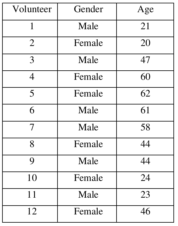
Pairing consecutive volunteers by age (without regard to gender) gives the six blocks:
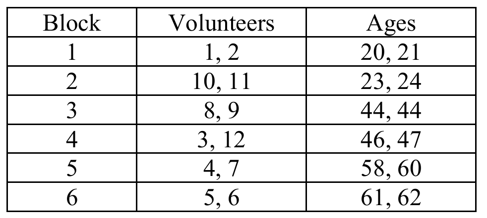
Since these researchers believe that the condition of hair changes with age but not gender, the volunteers are sorted from youngest to oldest. The volunteers in the sorted list are paired to form six blocks of size two. More specifically, the youngest two volunteers are placed in the first block. The next two volunteers in the sorted list are placed in the second block. This pairing continues until all six blocks of two are formed, with the oldest two volunteers in the sixth block.
(b)
Since both age and gender are believed to affect hair condition, volunteers must be blocked so that each block contains two people of the same gender and similar age.
First, separate by gender, then sort each group by age and pair consecutively
Males sorted by age: Volunteer 1 (age 21), Volunteer 11 (age 23), Volunteer 9 (age 44), Volunteer 3 (age 47), Volunteer 7 (age 58), Volunteer 6 (age 61)
Females sorted by age: Volunteer 2 (age 20), Volunteer 10 (age 24), Volunteer 8 (age 44), Volunteer 12 (age 46), Volunteer 4 (age 60), Volunteer 5 (age 62)
The six blocks are:
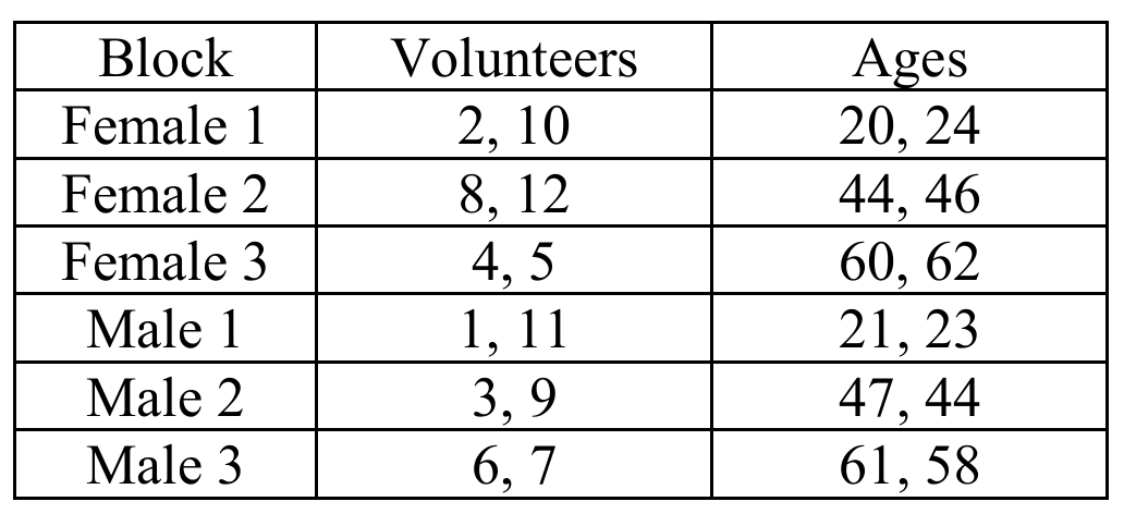
Since these researchers believe that the condition of hair changes with both age and gender, the women are sorted from youngest to oldest and then the men are sorted from youngest to oldest. The women (men) in the sorted list are paired to form the blocks of size two. More specifically, the youngest two women (men) are placed in a block. The next two youngest women (men) are placed in another block. Finally, the oldest two women (men) are placed in another block.
(c)
No, this is not an appropriate method for assigning treatments. Assigning the new formula to three entire blocks and the current formula to three other blocks does not allow a fair within-block comparison, because within each block both members would receive the same formula.
The correct approach in a matched-pairs block design is to randomly assign one person within each block to the new formula and the other to the current formula. This can be done as follows:
For each of the six blocks, flip a fair coin (or use a random number table/generator). If the result is heads (or the random digit is 0–4), assign the lower-numbered volunteer to the new formula and the other to the current formula. If tails (or digit 5–9), reverse the assignment. This ensures that within every block, one person receives the new formula and one receives the current formula, making a valid matched comparison possible.
\(\boxed{\text{Randomly assign one person per block to new formula; other receives current formula}}\)
Question
Most-appropriate topic codes (AP Statistics):
• Topic 1.11 — Random Sampling (Part c)
• Topic 1.12 — Potential Problems with Sampling (Part c)
▶️ Answer/Explanation
(a)
If volunteers who work together are all placed in the same program, there’s a risk that something specific to their workplace situation gets mixed up with the effect of the program itself. For example, suppose this group’s department recently had a deadline pushed back, which on its own would lower everyone’s stress level in that department regardless of which program they’re doing. If this entire group ends up in, say, the tai chi group, then the drop in stress they experience could mistakenly be credited to tai chi, when really it was caused by the lighter workload.
Random assignment fixes this issue. By randomly assigning volunteers to the two programs instead of letting groups choose, we spread people from this department across both the tai chi and yoga groups. This way, any unusual circumstance affecting that department’s stress levels — like the deadline change — gets “evened out” between the two treatment groups rather than being concentrated in just one. Randomization helps make sure the two groups are comparable at the start, so that any difference we see at the end can be attributed to the program rather than to some other confounding factor.
(b)
Yes, a control group would add useful information. Without one, the company could only compare tai chi to yoga directly — they could say which of the two programs led to a bigger drop in stress, but they couldn’t say whether either program actually caused a reduction in stress at all.
Here’s the issue: stress levels might naturally go down over a \(10\)-week period for reasons that have nothing to do with either program — for instance, if the overall work environment becomes less hectic during that time, everyone’s stress might drop a little just from that. A control group, which doesn’t participate in either program but still has its stress measured at the start and end of the \(10\) weeks, gives a baseline for what “no treatment” looks like under those same conditions.
By comparing each treatment group’s change in stress to the control group’s change, the company can tell how much of the reduction is actually attributable to tai chi or yoga specifically, rather than just background changes that would have happened anyway.
(c)
No, it is not reasonable to generalize these findings to all employees of the company. The participants in this study were volunteers, not a random sample of employees. People who choose to volunteer for a stress-reduction study might already be different from the typical employee — for example, they might be more motivated to manage their stress, more open to trying tai chi or yoga, or have more flexible schedules that let them give up part of their lunch hour.
Because the group wasn’t randomly selected from the entire employee population, there’s no guarantee that what works (or doesn’t work) for these volunteers would apply the same way to employees who didn’t volunteer. So while the random assignment within the study supports drawing cause-and-effect conclusions about tai chi versus yoga for people like these volunteers, it doesn’t justify extending those conclusions to the company as a whole.
Question
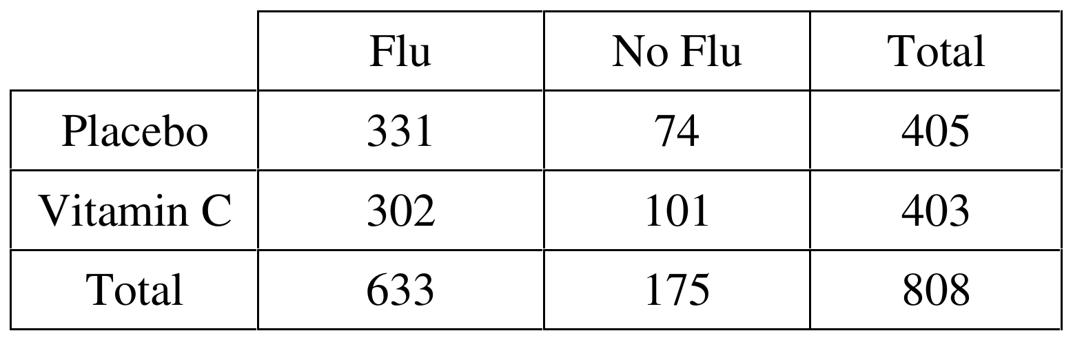
Most-appropriate topic codes (AP Statistics):
• Topic 3.12 — Setting Up a Test for the Difference Between Two Population Proportions (Part b)
• Topic 3.13 — Carrying Out a Test for the Difference Between Two Population Proportions (Part b)
• Topic 3.9 — Sampling Distributions for the Difference Between Sample Proportions (Part b)
▶️ Answer/Explanation
(a)
This study is an experiment, not an observational study.
In an experiment, the researchers deliberately impose a treatment on the subjects — here, the researchers assigned subjects to either the vitamin C group or the placebo group, rather than simply observing what subjects naturally chose to do.
Crucially, subjects were randomly assigned to the two treatment groups, which is the hallmark of a well-designed experiment and allows for causal conclusions to be drawn.
The use of a placebo and blind evaluation by a physician further strengthen this as a controlled experiment.
(b)
The health expert could use a two-proportion \(z\)-test to support this claim.
Let \(p_T\) be the true proportion of students (in the population of volunteers) who contract the flu when taking vitamin C, and let \(p_C\) be the true proportion who contract the flu when taking a placebo.
The hypotheses are:
\( H_0: p_T – p_C = 0 \quad \text{(vitamin C has no effect on flu occurrence)} \)
\( H_a: p_T – p_C < 0 \quad \text{(vitamin C reduces flu occurrence)} \)
Equivalently, this can be written as \(H_0: p_T = p_C\) versus \(H_a: p_T < p_C\), where a one-sided alternative is used because the claim is specifically that vitamin C reduces the occurrence of flu.
Question
Most-appropriate topic codes (AP Statistics):
• Topic 4.10 — Carrying Out a Test for the Difference Between Two Population Means (Part c)
• Topic 4.9 — Setting Up a Test for the Difference Between Two Population Means (Part c)
▶️ Answer/Explanation
(a)
Assign each of the 300 subjects a unique number from 001 to 300.
Use a random number table or a random number generator to randomly select 150 of these numbers — the subjects corresponding to those numbers will be placed in the experimental group (new filter), and the remaining 150 subjects will be assigned to the control group (standard filter).
This ensures that each subject has an equal chance of being assigned to either group, and that both groups end up with exactly 150 subjects.
(b)
Without a control group, if cholesterol levels change over the 10-week period, there is no way to know whether the change was caused by the new filter or by some other factor that changed during that time — for example, seasonal changes in diet or physical activity.
Simply measuring cholesterol at the beginning and end for one group only tells us that a change occurred, but not why it occurred.
By including a control group using the standard filter, researchers can compare the mean change in cholesterol between the two groups, allowing them to attribute any difference specifically to the new filter rather than to an outside confounding variable.
In short, the control group is what makes it possible to isolate the effect of the new filter from other changes that might naturally occur over the 10-week period.
(c)
The appropriate test is the two-sample \(t\)-test for means (or equivalently, the two-sample \(t\)-test for mean differences).
This test compares the mean change in cholesterol level for the new-filter group against the mean change in cholesterol level for the standard-filter group, using two independent samples of size 150 each.
(d)
Smoking is known to be related to cholesterol level, so if the study included both smokers and nonsmokers, smoking status could act as an extraneous source of variability — making it harder to detect the true effect of the coffee filter.
By restricting the study to nonsmokers only, the researchers create more homogeneous groups, reducing variability within each group and allowing for a more precise and sensitive comparison of the filter’s effect on cholesterol.
This is similar in spirit to blocking — controlling for a known nuisance variable (smoking) so that it does not obscure the treatment effect, though it does mean the results can only be generalized to nonsmokers.