▶️ Answer/Explanation
(a)
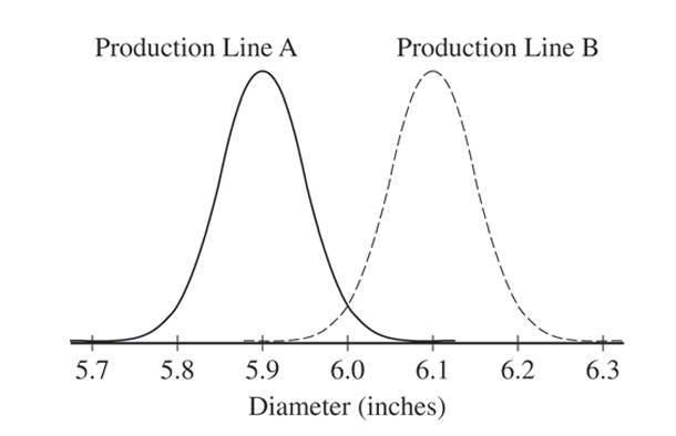
No. Method 2 samples from only one production line. Since the two lines produce tortillas with different mean diameters (\(5.9\) vs \(6.1\) inches), a sample from just one line cannot represent the entire population from both lines.
(b)
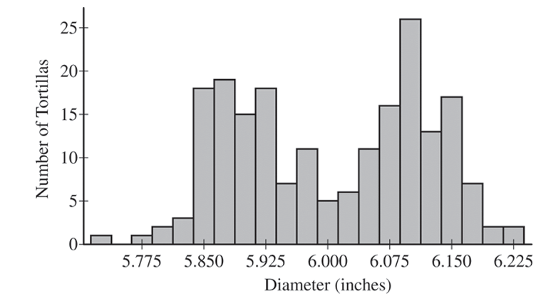
Method 1 was likely used. The histogram is bimodal, suggesting the sample contains tortillas from both production lines (centered near \(5.9\) and \(6.1\) inches). Method 2 would likely produce a unimodal histogram.
(c)
Method 2 will result in less variability within a single sample. Method 2 samples from only one distribution (either Line A or Line B), while Method 1 samples from a mixture of two distributions with different centers, leading to greater spread in the combined sample data.
(d)
For Method 1 (\(n=200\), \(\mu=6\), \(\sigma=0.11\)):
- Shape: Approximately normal (by CLT, since \(n=200 \ge 30\)).
- Center: Mean \(\mu_{\bar{x}} = \mu = 6\) inches.
- Spread: Standard deviation \(\sigma_{\bar{x}} = \frac{\sigma}{\sqrt{n}} = \frac{0.11}{\sqrt{200}} \approx 0.0078\) inches.
(e)
Method 1 will result in less variability in the \(365\) daily sample means.
Explanation: Sample means from Method 1 will cluster tightly around \(6\) inches (small \(\sigma_{\bar{x}}\)). Sample means from Method 2 will cluster around \(5.9\) inches about half the time and around \(6.1\) inches the other half, resulting in a much wider spread of the \(365\) sample means.
(f)
Method 1 is more likely to produce a sample mean close to \(6\) inches.
Explanation: Although both methods yield unbiased estimates in the long run, Method 1 has a sampling distribution with significantly less variability (as shown in (d) and (e)) and is centered exactly at \(6\). Therefore, any single sample mean from Method 1 is much more likely to be near \(6\) than a sample mean from Method 2, which will likely be near \(5.9\) or \(6.1\).