AP Statistics 1.7 Summary Statistics for a Quantitative Variable- FRQs - Exam Style Questions

Question

A company sells a certain type of whistle. The price of the whistle varies from store to store. Julio, a statistician at the company, wants to estimate the mean price, in dollars ($\$$), of this type of whistle at all stores that sell the whistle.

(a) (i) Identify the appropriate inference procedure for Julio to use.

(ii) Describe the parameter for the inference procedure you identified in part (a-i) in context.

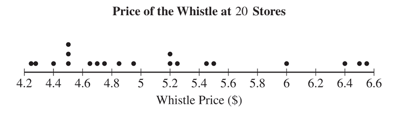
Julio called the managers of $20$ randomly selected stores that sell the whistle and recorded the price of the whistle at each store. Following is a dotplot of Julio’s data.

The summary statistics for Julio’s data are shown in the following table.

Sample Size	Mean	Std Dev	Min	$Q_1$	Median	$Q_3$	Max
$20$	$5.12$	$0.743$	$4.25$	$4.51$	$4.885$	$5.475$	$6.58$

(b) Julio wants to examine some characteristics of the distribution of the sample of whistle prices.
(i) Describe the shape of the distribution of the sample of whistle prices. Justify your response using appropriate values from the summary statistics table.
(ii) Using the $1.5 \times IQR$ rule, determine whether there are any outliers in the sample of whistle prices. Justify your response.

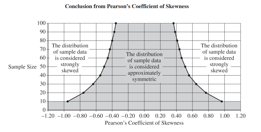
It can often be difficult to determine whether the distribution of sample data is skewed by looking at a graph of the data and the summary statistics, particularly when the sample size is small. Thus, statisticians sometimes measure how skewed a data set is. One such measure is Pearson’s coefficient of skewness, which is calculated using the following formula.

\[ \text{Pearson’s Coefficient of Skewness} \;=\; \frac{3\!\left(\bar{x}-m\right)}{s} \]

In the formula, $\bar{x}$ is the sample mean, $m$ is the sample median, and $s$ is the sample standard deviation.

(c) (i) Calculate Pearson’s coefficient of skewness for Julio’s sample of $20$ whistle prices. Show your work.
(ii) Indicate the value of the Pearson’s coefficient of skewness you calculated in part (c-i) for the appropriate sample size by marking it with an “X” on the preceding graph.

(d) Consider your work in part (c).
(i) What should you conclude about the shape of the distribution of the sample of whistle prices? Justify your response.

Julio’s inference procedure in part $(a\text{-}i)$ needs one of the following requirements to be satisfied to verify the normality condition.

The sample size is greater than or equal to $30$.
If the sample size is less than $30$, the distribution of the sample data is not strongly skewed and does not have outliers.

(ii) Using your response to (d-i) and the preceding requirements, is the normality condition satisfied for Julio’s data? Explain your response.

Most-appropriate topic codes (CED):

• TOPIC 7.2: Constructing a Confidence Interval for a Population Mean
• TOPIC 1.6: Describing the Distribution of a Quantitative Variable
• TOPIC 1.7: Summary Statistics for a Quantitative Variable

▶️ Answer/Explanation

Detailed solution

(a)
(i) The appropriate inference procedure is a one-sample t-interval for a population mean.
(ii) The parameter of interest is $\mu$, the true mean price, in dollars, of this type of whistle at all stores that sell the whistle.

(b)
(i) The distribution of the sample of whistle prices appears to be slightly skewed to the right. This is because the sample mean ($5.12$) is greater than the sample median ($4.885$).
(ii) First, calculate the IQR: $IQR = Q_3 – Q_1 = 5.475 – 4.51 = 0.965$.
Next, calculate the outlier fences:
– Lower Fence: $Q_1 – 1.5(IQR) = 4.51 – 1.5(0.965) = 3.0625$
– Upper Fence: $Q_3 + 1.5(IQR) = 5.475 + 1.5(0.965) = 6.9225$
Since the minimum value ($4.25$) is greater than the lower fence and the maximum value ($6.58$) is less than the upper fence, there are **no outliers** in the sample.

(c)
(i) Pearson’s Coefficient of Skewness = $\frac{3(\bar{x} – m)}{s} = \frac{3(5.12 – 4.885)}{0.743} \approx 0.949$.
(ii) An “X” is marked on the graph at the coordinate ($0.949, 20$).

(d)
(i) Based on the graph, the point ($0.949, 20$) falls into the region labeled “The distribution of sample data is considered strongly skewed.”
(ii) No, the normality condition is not satisfied. The sample size ($n=20$) is not greater than or equal to $30$, and the analysis in part (d-i) shows that the distribution of the sample data is strongly skewed.

AP Statistics 1.7 Summary Statistics for a Quantitative Variable- FRQs - Exam Style Questions

Question

Resources

Members

Company