AP Statistics 1.8 Graphical Representations of Summary Statistics- FRQs - Exam Style Questions

(a)
From the histogram for streams colder than \( 8^\circ \mathrm{C} \):
• Shape: Unimodal and skewed left (longer tail toward lower values \( \approx 2\text{–}6 \,\mathrm{mg}/\ell \)).
• Center: Median between \( 11 \) and \( 12 \,\mathrm{mg}/\ell \) (tallest bars around \( 10\text{–}12 \)).
• Spread: Approximate range \( \approx 14 – 2 = 12 \,\mathrm{mg}/\ell \). Quartiles appear near \( Q_1 \in (10,11) \) and \( Q_3 \in (12,13) \), so \( \mathrm{IQR} \approx 2 \,\mathrm{mg}/\ell \).
• Unusual features: Several potential low outliers in the \( 2\text{–}3 \), \( 4\text{–}5 \), and \( 5\text{–}6 \) bins because these are far below \( Q_1 – 1.5\,\mathrm{IQR} \approx 10 – 1.5(2) = 7 \,\mathrm{mg}/\ell \).
Therefore, the distribution is described as unimodal, skewed left, with median \( 11\text{–}12 \,\mathrm{mg}/\ell \), IQR \( \approx 2 \,\mathrm{mg}/\ell \), and possible low outliers.

(b)
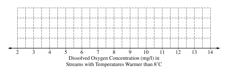
Use the five-number summary to draw the boxplot for warmer than \( 8^\circ \mathrm{C} \):
• Minimum \( = 2.10 \), \( Q_1 = 4.39 \), Median \( = 5.43 \), \( Q_3 = 6.12 \), Maximum \( = 13.45 \).
• Compute \( \mathrm{IQR} = Q_3 – Q_1 = 6.12 – 4.39 = 1.73 \).
• Fences for outliers (not drawn, but for reference): lower \( Q_1 – 1.5\mathrm{IQR} = 4.39 – 1.5(1.73) = 1.885 \) (so \( 2.10 \) is not beyond the fence); upper \( Q_3 + 1.5\mathrm{IQR} = 6.12 + 1.5(1.73) = 8.715 \) (values above this would be flagged, but the instruction says not to indicate outliers).
• The box spans \( 4.39 \) to \( 6.12 \) with a median line at \( 5.43 \); whiskers extend to \( 2.10 \) (left) and \( 13.45 \) (right).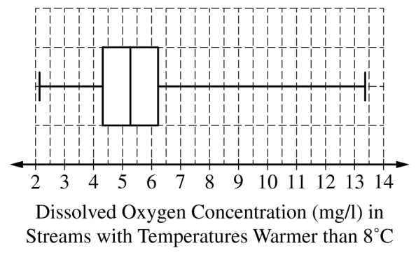

(c)
If higher dissolved oxygen implies healthier streams, then colder streams are generally healthier because:
• Center comparison: Colder streams have a larger center (median between \( 11 \) and \( 12 \,\mathrm{mg}/\ell \)) than warmer streams (median \( 5.43 \,\mathrm{mg}/\ell \)).
• Shape: Colder distribution is skewed left (most values high with a few small ones), whereas the warmer distribution is right-skewed given the very long upper whisker to \( 13.45 \).
• Spread: Both show similar middle-spread (colder \( \mathrm{IQR} \approx 2 \,\mathrm{mg}/\ell \); warmer \( \mathrm{IQR} = 1.73 \,\mathrm{mg}/\ell \)), but this does not overturn the much higher center for colder streams.
Hence, using center (and acknowledging shape and spread), colder streams better satisfy the researchers’ criterion.