AP Statistics 2.10 The Binomial Distribution- Exam Style Questions - FRQs - New Syllabus

Question

Ms. Fey is a manager at a restaurant. To improve the dining experience for her customers, she uses a digital music service to create a playlist of songs that will be played in the restaurant. The playlist contains 1,000 songs and consists of four different types of music in the following quantities: 200 country songs, 400 pop songs, 100 rock songs, and 300 jazz songs. The digital music service will select songs at random from the playlist to be played in the restaurant. Any song can be replayed at any time.

i. Suppose one song is selected at random to be played. What is the probability that the song is a rock song? Show your work.
ii. Suppose two songs are selected at random to be played. What is the probability that both songs are rock songs? Show your work.

B. In every one-hour period, 20 songs will be played at random and any song can be replayed at any time. Ms. Fey is interested in how many rock songs will be played in a typical one-hour period.

i. Define the random variable of interest to Ms. Fey, and state how the random variable is distributed.
ii. What is the expected value for the random variable in part B (i)? Show your work.

C. Recall that in every one-hour period, 20 songs will be played at random and any song can be replayed at any time.

i. Determine the probability that 4 or more rock songs in a particular one-hour period will be played. Show your work.
ii. Suppose 4 rock songs are played during a particular one-hour period. Does this provide strong evidence that the song selection process was not truly random? Justify your answer without performing an inference procedure.

Most-appropriate topic codes (AP Statistics):

• Topic $2.4$ — Introduction to Probability (Part $ \mathrm{A} $)
• Topic $2.7$ — Independent Events and Unions of Events (Part $ \mathrm{A} $)
• Topic $2.10$ — The Binomial Distribution (Parts $ \mathrm{B} $, $ \mathrm{C} $)

▶️ Answer/Explanation

A. i.
Let $R$ represent selecting a rock song.
$P(R) = \dfrac{\text{Number of rock songs}}{\text{Total number of songs}} = \dfrac{100}{1,000}$
$\boxed{P(R) = 0.10}$

A. ii.
Because any song can be repeated, the selection of the second song is independent of the first.
$P(\text{Both Rock}) = P(R) \times P(R) = 0.10 \times 0.10$
$\boxed{P(\text{Both Rock}) = 0.01}$

B. i.
• Let $X$ be the random variable representing the number of rock songs played in a one-hour period.
• The random variable $X$ follows a binomial distribution, expressed as $X \sim \text{Binomial}(n = 20, p = 0.10)$.

B. ii.
The expected value of a binomial distribution is given by the formula $E(X) = n \cdot p$.
$E(X) = 20 \times 0.10$
$\boxed{E(X) = 2\text{ songs}}$

C. i.
We want to calculate $P(X \ge 4) = 1 – P(X \le 3)$.
Using the binomial cumulative distribution formula, $P(X \le 3) = \sum_{k=0}^{3} \binom{20}{k} (0.10)^k (0.90)^{20-k} \approx 0.8670$.
$P(X \ge 4) = 1 – 0.8670$
$\boxed{P(X \ge 4) = 0.1330}$

C. ii.
• No, this does not provide strong evidence that the song selection process was not truly random.
• The calculated probability of playing 4 or more rock songs is $0.1330$, which is greater than conventional significance thresholds like $\alpha = 0.05$, meaning an outcome of 4 rock songs is a relatively common chance occurrence.

Question

A machine at a manufacturing company is programmed to fill shampoo bottles such that the amount of shampoo in each bottle is normally distributed with mean 0.60 liter and standard deviation 0.04 liter. Let the random variable A represent the amount of shampoo, in liters, that is inserted into a bottle by the filling machine.

(a) A bottle is considered to be underfilled if it has less than 0.50 liter of shampoo. Determine the probability that a randomly selected bottle of shampoo will be underfilled. Show your work.

After the bottles are filled, they are placed in boxes of 10 bottles per box. After the bottles are placed in the boxes, several boxes are placed in a crate for shipping to a beauty supply warehouse. The manufacturing company’s contract with the beauty supply warehouse states that one box will be randomly selected from a crate. If 2 or more bottles in the selected box are underfilled, the entire crate will be rejected and sent back to the manufacturing company.

(b) The beauty supply warehouse manager is interested in the probability that a crate shipped to the warehouse will be rejected. Assume that the amounts of shampoo in the bottles are independent of each other.

(i) Define the random variable of interest for the warehouse manager and state how the random variable is distributed.
(ii) Determine the probability that a crate will be rejected by the warehouse manager. Show your work.

To reduce the number of crates rejected by the beauty supply warehouse manager, the manufacturing company is considering adjusting the programming of the filling machine so that the amount of shampoo in each bottle is normally distributed with mean 0.56 liter and standard deviation 0.03 liter.

(c) Would you recommend that the manufacturing company use the original programming of the filling machine or the adjusted programming of the filling machine? Provide a statistical justification for your choice.

Most-appropriate topic codes (AP Statistics):

• Topic $2.10$ — The Binomial Distribution (Part $ \mathrm{b} $)
• Topic $2.11$ — The Normal Distribution (Parts $ \mathrm{a} $, $ \mathrm{c} $)

▶️ Answer/Explanation

(a)
Let $A$ be the amount of shampoo in a bottle. We need to find $P(A < 0.50)$.
$z = \frac{0.50 – 0.60}{0.04} = -2.5$
$P(A < 0.50) = P(Z < -2.5) = 0.0062$

(b)(i)
Let $X$ represent the number of underfilled bottles in a randomly selected box of 10 bottles. Because each bottle’s volume is independent and has the same probability of being underfilled, the random variable $X$ has a binomial distribution with $n = 10$ trials and probability of success $p = 0.0062$.

(b)(ii)
The probability that a crate will be rejected is the probability of finding 2 or more underfilled bottles in a box: $P(X \ge 2)$.
$P(X \ge 2) = 1 – P(X \le 1) = 1 – [P(X = 0) + P(X = 1)]$
$P(X \ge 2) = 1 – \left[\binom{10}{0}(0.0062)^0(0.9938)^{10} + \binom{10}{1}(0.0062)^1(0.9938)^9\right]$
$P(X \ge 2) \approx 1 – [0.9397 + 0.0586] \approx 1 – 0.9983 = 0.0017$

(c)
Under the adjusted programming, the new mean is $0.56$ and the standard deviation is $0.03$. The new probability of a bottle being underfilled is:
$z = \frac{0.50 – 0.56}{0.03} = -2.0$
$P(Z < -2.0) \approx 0.02275$
Because the probability of an underfilled bottle is much greater for the adjusted programming ($0.0228$) than for the original programming ($0.0062$), the manufacturing company should keep the original programming. Using the adjusted settings would actually result in more underfilled bottles, thereby increasing the number of rejected crates.

Question

To increase morale among employees, a company began a program in which one employee is randomly selected each week to receive a gift card. Each of the company’s $200$ employees is equally likely to be selected each week, and the same employee could be selected more than once. Each week’s selection is independent from every other week.

(a) Consider the probability that a particular employee receives at least one gift card in a $52$-week year.

i. Define the random variable of interest and state how the random variable is distributed.
ii. Determine the probability that a particular employee receives at least one gift card in a $52$-week year. Show your work.

(b) Calculate and interpret the expected value for the number of gift cards a particular employee will receive in a $52$-week year. Show your work.

(c) Suppose that Agatha, an employee at the company, never receives a gift card for an entire $52$-week year. Based on her experience, does Agatha have a strong argument that the selection process was not truly random? Explain your answer.

Most-appropriate topic codes (AP Statistics):

• Topic $2.10$ — The Binomial Distribution (Parts $ \mathrm{a} $, $ \mathrm{b} $, $ \mathrm{c} $)

▶️ Answer/Explanation

(a)(i)
Let $X$ be the number of gift cards a specific employee receives in a $52$-week year.
Since the probability of winning is constant ($p = \frac{1}{200} = 0.005$) and the weekly drawings are independent, $X$ follows a binomial distribution with $n = 52$ trials and probability of success $p = 0.005$.

(a)(ii)
To find the probability of winning at least once, it’s easiest to use the complement rule (1 minus the probability of winning zero times):
$ P(X \ge 1) = 1 – P(X = 0) $
$ P(X \ge 1) = 1 – \binom{52}{0}(0.005)^0(0.995)^{52} $
$ P(X \ge 1) = 1 – 0.7705 $
$ P(X \ge 1) = 0.2295 $

(b)
The expected value (mean) for a binomial distribution is calculated as $\mu = np$.
$ E(X) = 52 \times 0.005 = 0.26 $
This means that if we repeat this $52$-week selection process for many, many years, a specific employee will receive an average of about $0.26$ gift cards per year (or roughly one card every four years).

(c)
No, Agatha does not have a strong argument.
As we found in the earlier calculations, the probability of getting zero gift cards in a year is $P(X = 0) \approx 0.7705$.
Because there is roughly a $77\%$ chance of walking away empty-handed in a perfectly fair system, her experience of not winning is highly likely and completely consistent with a truly random process.

Question

A medical researcher surveyed a large group of men and women about whether they take medicine as prescribed.

The responses were categorized as never, sometimes, or always. The relative frequency of each category is shown in the table.

(a) One person from those surveyed will be selected at random.

i. What is the probability that the person selected will be someone whose response is never and who is a woman?

ii. What is the probability that the person selected will be someone whose response is never or who is a woman?

iii. What is the probability that the person selected will be someone whose response is never given that the person is a woman?

(b) For the people surveyed, are the events of being a person whose response is never and being a woman independent? Justify your answer.

(c) Assume that, in a large population, the probability that a person will always take medicine as prescribed is $0.54$. If $5$ people are selected at random from the population, what is the probability that at least $4$ of the people selected will always take medicine as prescribed? Support your answer.

Most-appropriate topic codes (AP Statistics):

• Topic $2.6$ — Conditional Probability (Part $ \mathrm{a} $)
• Topic $2.7$ — Independent Events and Mutually Exclusive Events (Part $ \mathrm{b} $)
• Topic $2.10$ — The Binomial Distribution (Part $ \mathrm{c} $)

▶️ Answer/Explanation

(a)(i)
From the given two-way table, we can find the joint probability directly by looking at the intersection of the “Women” row and “Never” column.
$P(\text{never and woman}) = 0.0636$

(a)(ii)
To find this probability, we use the general addition rule by adding the marginal probability of “never” to the marginal probability of “woman”, and subtracting their intersection.
$P(\text{never or woman}) = P(\text{never}) + P(\text{woman}) – P(\text{never and woman})$
$P(\text{never or woman}) = 0.1200 + 0.5300 – 0.0636 = 0.5864$

(a)(iii)
For conditional probability, we divide the joint probability of both events occurring by the marginal probability of the given condition (“woman”).
$P(\text{never} \mid \text{woman}) = \dfrac{P(\text{never and woman})}{P(\text{woman})}$
$P(\text{never} \mid \text{woman}) = \dfrac{0.0636}{0.5300} = 0.12$

(b)
We can check for independence by seeing if the conditional probability of an event equals its marginal probability.
Since $P(\text{never} \mid \text{woman}) = 0.12$ and the overall probability $P(\text{never}) = 0.12$, the probabilities are identical.
Yes, this indicates that the event of responding “never” is perfectly independent of the event of being a “woman”.

(c)
This scenario can be modeled using a binomial distribution with $n=5$ trials and a success probability of $p=0.54$.
We need to find the probability of getting at least $4$ successes, which means finding the sum of $P(X=4)$ and $P(X=5)$.
$P(X \ge 4) = \binom{5}{4}(0.54)^4(0.46)^1 + \binom{5}{5}(0.54)^5(0.46)^0$
$P(X \ge 4) \approx 0.19557 + 0.04592 \approx 0.24149$

Question

Approximately $3.5$ percent of all children born in a certain region are from multiple births (that is, twins, triplets, etc.). Of the children born in the region who are from multiple births, $22$ percent are left-handed. Of the children born in the region who are from single births, $11$ percent are left-handed.

(a) What is the probability that a randomly selected child born in the region is left-handed?

(b) What is the probability that a randomly selected child born in the region is a child from a multiple birth, given that the child selected is left-handed?

(c) A random sample of $20$ children born in the region will be selected. What is the probability that the sample will have at least $3$ children who are left-handed?

Most-appropriate topic codes (AP Statistics):

• Topic $2.6$ — Conditional Probability (Parts $ \mathrm{a} $, $ \mathrm{b} $)
• Topic $2.7$ — Independent Events and Mutually Exclusive Events (Parts $ \mathrm{a} $, $ \mathrm{b} $)
• Topic $2.10$ — The Binomial Distribution (Part $ \mathrm{c} $)

▶️ Answer/Explanation

(a)
Let $L$ denote the event that a child is left-handed, $M$ denote the event of a multiple birth, and $S$ denote the event of a single birth.
We are given: $P(M) = 0.035$, $P(S) = 0.965$, $P(L \mid M) = 0.22$, and $P(L \mid S) = 0.11$.
Apply the Law of Total Probability:
$P(L) = P(M) \cdot P(L \mid M) + P(S) \cdot P(L \mid S)$
$P(L) = (0.035)(0.22) + (0.965)(0.11)$
$P(L) = 0.0077 + 0.10615$
$\boxed{P(L) = 0.11385}$
Think of this as a weighted average of the two left-handedness rates — you weight each group’s rate by how large that group is. Since single births make up the overwhelming majority (96.5%), they drive the overall rate, which lands very close to 11%. The small multiple-birth group nudges it up just slightly to about 11.4%.

(b)
We use the definition of conditional probability to find $P(M \mid L)$.
$P(M \mid L) = \dfrac{P(M \cap L)}{P(L)}$
The joint probability $P(M \cap L)$ is found using the multiplication rule:
$P(M \cap L) = P(M) \cdot P(L \mid M) = (0.035)(0.22) = 0.0077$
Using $P(L) = 0.11385$ from part (a):
$P(M \mid L) = \dfrac{0.0077}{0.11385}$
$\boxed{P(M \mid L) \approx 0.0676}$
This is a classic Bayes-style reversal — we flipped from “given multiple birth, what’s the chance of being left-handed?” to “given left-handed, what’s the chance of multiple birth?” Even though multiple-birth children are twice as likely to be left-handed (22% vs. 11%), they are so rare (only 3.5% of all births) that among all left-handed children, only about 6.8% actually come from multiple births. Rarity wins.

(c)
Let $X$ represent the number of left-handed children in a random sample of $20$. Since each child is selected independently with the same probability of being left-handed, $X$ follows a binomial distribution:
$X \sim \operatorname{Binomial}(n = 20,\; p = 0.11385)$
We want $P(X \geq 3)$. Using the complement:
$P(X \geq 3) = 1 – P(X \leq 2) = 1 – \bigl[P(X = 0) + P(X = 1) + P(X = 2)\bigr]$
Using the binomial formula $\displaystyle P(X = k) = \binom{20}{k}(0.11385)^{k}(0.88615)^{20-k}$:
$P(X = 0) = \dbinom{20}{0}(0.11385)^{0}(0.88615)^{20} \approx 0.0891$
$P(X = 1) = \dbinom{20}{1}(0.11385)^{1}(0.88615)^{19} \approx 0.2289$
$P(X = 2) = \dbinom{20}{2}(0.11385)^{2}(0.88615)^{18} \approx 0.2797$
Summing the complement terms:
$P(X \leq 2) \approx 0.0891 + 0.2289 + 0.2797 = 0.5977$
$P(X \geq 3) = 1 – 0.5977$
$\boxed{P(X \geq 3) \approx 0.402}$
The complement trick is your best friend here — instead of adding up $P(X=3) + P(X=4) + \cdots + P(X=20)$, which would take forever, you subtract the small pile of easy cases (0, 1, or 2 left-handed kids) from 1. With only about an 11.4% chance per child, there’s roughly a 40% chance that 3 or more kids in a group of 20 will be left-handed — higher than you might expect, because “at least 3” covers most of the distribution.

Question

An airline claims that there is a $0.10$ probability that a coach-class ticket holder who flies frequently will be upgraded to first class on any flight. This outcome is independent from flight to flight. Sam is a frequent flier who always purchases coach-class tickets.

(a) What is the probability that Sam’s first upgrade will occur after the third flight?

(b) What is the probability that Sam will be upgraded exactly $2$ times in his next $20$ flights?

(c) Sam will take $104$ flights next year. Would you be surprised if Sam receives more than $20$ upgrades to first class during the year? Justify your answer.

Most-appropriate topic codes (AP Statistics):

• Topic 2.10 — The Binomial Distribution (Parts b & c)
• Topic 2.10 — The Binomial Distribution (Part a)
• Topic 2.7 — Independent Events and Unions of Events (Part a)

▶️ Answer/Explanation

(a)
Let $Y$ denote the number of flights Sam must make until he receives his first upgrade. The random variable $Y$ follows a geometric distribution with $p = 0.1$.
The probability that Sam’s upgrade will occur after his third flight is equivalent to the probability that he receives no upgrade on his first three flights.
$P(Y \ge 4) = 1 – P(Y \le 3)$
$= 1 – [P(Y=1) + P(Y=2) + P(Y=3)]$
$= 1 – [0.1 + 0.9(0.1) + (0.9)^2(0.1)]$
$= 1 – [0.1 + 0.09 + 0.081]$
$= 0.729$
$\boxed{0.729}$

(b)
Let $X$ denote the number of upgrades Sam will receive in $20$ flights. The random variable $X$ follows a binomial distribution with $n = 20$ independent trials and $p = 0.1$.
The probability that Sam will be upgraded exactly $2$ times is calculated as follows:
$P(X = 2) = \binom{20}{2}(0.1)^2(0.9)^{18}$
$\approx 0.2852$
$\boxed{P(X = 2) \approx 0.2852}$

(c)
Let $X$ denote the number of upgrades Sam will receive in $104$ flights. The random variable $X$ follows a binomial distribution with $n = 104$ independent trials and $p = 0.1$.
We need to find the probability of receiving more than $20$ upgrades:
$P(X > 20) = 1 – P(X \le 20)$
$\approx 1 – 0.9986$
$\approx 0.0014$
Because this probability is so small (less than $1\%$), it is very unlikely that Sam would receive more than $20$ upgrades in $104$ flights if the airline’s claim is correct. This would be expected to happen less than $1$ percent of the time.
Therefore, I would be surprised if Sam receives more than $20$ upgrades during the year.

Question

An automobile company wants to learn about customer satisfaction among the owners of five specific car models. Large sales volumes have been recorded for three of the models, but the other two models were recently introduced so their sales volumes are smaller. The number of new cars sold in the last six months for each of the models is shown in the table below.

The company can obtain a list of all individuals who purchased new cars in the last six months for each of the five models shown in the table. The company wants to sample 2,000 of these owners.

(a) For simple random samples of 2,000 new car owners, what is the expected number of owners of model E and the standard deviation of the number of owners of model E?

(b) When selecting a simple random sample of 2,000 new car owners, how likely is it that fewer than 12 owners of model E would be included in the sample? Justify your answer.

(c) The company is concerned that a simple random sample of 2,000 owners would include fewer than 12 owners of model D or fewer than 12 owners of model E. Briefly describe a sampling method for randomly selecting 2,000 owners that will ensure at least 12 owners will be selected for each of the 5 car models.

Most-appropriate topic codes (AP Statistics):

• Topic 2.8 — Introduction to Random Variables and Probability Distributions (Part a)
• Topic 2.10 — The Binomial Distribution (Parts a, b)
• Topic 1.11 — Random Sampling (Part c)

▶️ Answer/Explanation

(a)

Because the total population ($297,354$) is overwhelmingly large compared to the sample size ($2,000$), we can treat this as a binomial distribution even though sampling is without replacement.
The probability of selecting a model E owner is $p = \dfrac{2,323}{297,354} \approx 0.007812$.
The sample size is $n = 2000$.
Expected number (Mean):
$\mu_E = n \times p = 2000 \times 0.007812 \approx 15.62$ owners
Standard Deviation:
$\sigma_E = \sqrt{n \times p \times (1-p)} = \sqrt{2000 \times 0.007812 \times (1 – 0.007812)} = \sqrt{15.49} \approx 3.93$ owners

(b)

For the reason given in part (a), the binomial distribution with $n = 2,000$ and $p \approx 0.0078$ can be used here. The probability that the sample would contain fewer than 12 owners of model E is calculated from the binomial distribution to be $\sum_{x=0}^{11} \binom{2,000}{x} (0.0078)^x (0.9922)^{2,000-x} \approx 0.147$. This probability is small enough that the result (fewer than 12 owners of model E in the sample) is not likely, but this probability is also not small enough to consider the result very unlikely.

This binomial probability can also be evaluated using a normal approximation. This is reasonable because $n \times p = (2,000) \times (0.0078) = 15.6$ is larger than 10 and $n(1 – p) = (2,000) \times (0.9922) = 1,984.4$ is much larger than 10. Using the mean and standard deviation from part (a) gives

$P(X \le 11) \approx P\left( Z < \dfrac{12.0 – 15.62}{3.94} \right) = P(Z < -0.92) = 0.179$.

(c)

To guarantee at least 12 owners from each model, the company should use a stratified random sampling method.
The researcher should use the five car models as the strata.
They can determine how many individuals they want to sample from each model (stratum) as long as every model’s assigned sample size is $12$ or greater, and all five sizes add up to exactly $2,000$.
Then, they simply perform five separate simple random samples—one within each specific car model’s list of owners—to achieve the decided quota for that model.

Question

A test consisting of 25 multiple-choice questions with 5 answer choices for each question is administered. For each question, there is only 1 correct answer.

(a) Let $X$ be the number of correct answers if a student guesses randomly from the 5 choices for each of the 25 questions. What is the probability distribution of $X$?

This test, like many multiple-choice tests, is scored using a penalty for guessing. The test score is determined by awarding 1 point for each question answered correctly, deducting 0.25 point for each question answered incorrectly, and ignoring any question that is omitted. That is, the test score is calculated using the following formula.

$\text{Score} = (1 \times \text{number of correct answers}) – (0.25 \times \text{number of incorrect answers}) + (0 \times \text{number of omits})$

For example, the score for a student who answers 17 questions correctly, answers 3 questions incorrectly, and omits 5 questions is

$\text{Score} = (1 \times 17) – (0.25 \times 3) + (0 \times 5) = 16.25.$

(b) Suppose a student knows the correct answers for 18 questions, answers those 18 questions correctly, and chooses randomly from the 5 choices for each of the other 7 questions. Show that the expected value of the student’s score is 18 when using the scoring formula above.

(c) A score of at least 20 is needed to pass the test. Suppose a student knows the correct answers for 18 questions, answers those 18 questions correctly, and chooses randomly from the 5 choices for each of the other 7 questions. What is the probability that the student will pass the test?

Most-appropriate topic codes (AP Statistics):

• Topic $2.10$ — The Binomial Distribution (Parts $\mathrm{a}$, $\mathrm{b}$, $\mathrm{c}$)
• Topic $2.9$ — Parameters of Random Variables (Part $\mathrm{b}$)

▶️ Answer/Explanation

(a)
Since each question has 5 answer choices and only 1 is correct, the probability of guessing correctly on any single question is
$p = \frac{1}{5} = 0.20$
Each question is independent, and there are a fixed number of trials ($n = 25$), so $X$ follows a binomial distribution with parameters $n = 25$ and $p = 0.20$:
$X \sim B(25,\ 0.20)$
The probability mass function is:
$P(X = k) = \binom{25}{k}(0.20)^k(0.80)^{25-k}, \quad k = 0, 1, 2, \ldots, 25$
Think of it this way: every question is either right or wrong (two outcomes), the questions don’t affect each other (independence), there are exactly 25 of them (fixed $n$), and each one has the same $\frac{1}{5}$ chance of being correct — that’s the classic checklist for a binomial setup.

(b)
Let $Y$ be the number of correct guesses among the 7 randomly answered questions. Then
$Y \sim B(7,\ 0.20)$
The expected number of correct guesses is:
$E(Y) = np = 7 \times 0.20 = 1.4$
Since the student answers 7 questions randomly and gets $Y$ correct, the number answered incorrectly is $7 – Y$. The scoring formula gives:
$\text{Score} = (18 + Y) \times 1 – (7 – Y) \times 0.25 + 0$
$\text{Score} = 18 + Y – 1.75 + 0.25Y = 16.25 + 1.25Y$
Taking the expected value:
$E(\text{Score}) = E(16.25 + 1.25Y) = 16.25 + 1.25 \cdot E(Y)$
$E(\text{Score}) = 16.25 + 1.25 \times 1.4 = 16.25 + 1.75 = \boxed{18}$
The key insight here is that even though the student is guessing on 7 questions, the penalty for wrong answers exactly offsets the expected gain from lucky correct guesses — the expected score ends up right back at 18, the number the student knew for certain.

(c)
The student passes when $\text{Score} \geq 20$. Using the expression from part (b):
$16.25 + 1.25Y \geq 20$
$1.25Y \geq 3.75$
$Y \geq 3$
So the student needs to guess at least 3 of the 7 random questions correctly in order to pass. It’s easier to use the complement:
$P(Y \geq 3) = 1 – P(Y \leq 2)$
$P(Y \leq 2) = P(Y=0) + P(Y=1) + P(Y=2)$
$= \binom{7}{0}(0.2)^0(0.8)^7 + \binom{7}{1}(0.2)^1(0.8)^6 + \binom{7}{2}(0.2)^2(0.8)^5$
$= (0.8)^7 + 7(0.2)(0.8)^6 + 21(0.04)(0.8)^5$
$= 0.2097 + 0.3670 + 0.2753$
$= 0.8520$
Therefore:
$P(Y \geq 3) = 1 – 0.8520 = \boxed{0.148}$
There’s only about a 14.8% chance the student passes — which makes sense intuitively. Even though the expected score is exactly 18, passing requires being luckier than average on those 7 guesses, and the binomial distribution tells us that’s a relatively rare outcome.

Question

A tire manufacturer designed a new tread pattern for its all-weather tires. Repeated tests were conducted on cars of approximately the same weight traveling at 60 miles per hour. The tests showed that the new tread pattern enables the cars to stop completely in an average distance of 125 feet with a standard deviation of 6.5 feet and that the stopping distances are approximately normally distributed.

(a) What is the 70th percentile of the distribution of stopping distances?

(b) What is the probability that at least 2 cars out of 5 randomly selected cars in the study will stop in a distance that is greater than the distance calculated in part (a)?

(c) What is the probability that a randomly selected sample of 5 cars in the study will have a mean stopping distance of at least 130 feet?

Most-appropriate topic codes (AP Statistics):

• Topic $2.11$ — The Normal Distribution (Part $\mathrm{a}$)
• Topic $2.10$ — The Binomial Distribution (Part $\mathrm{b}$)
• Topic $2.12$ — Sampling Distributions and the Central Limit Theorem (Part $\mathrm{c}$)

▶️ Answer/Explanation

(a)
Let $X$ denote the stopping distance. We are told that $X$ is normally distributed with
$ \mu_X = 125 \text{ ft}, \qquad \sigma_X = 6.5 \text{ ft} $
We want the value $x$ such that $P(X \leq x) = 0.70$.
From the standard normal table, the $z$-score with a cumulative probability of $0.70$ is
$ z = 0.52 $
Using the $z$-score formula and solving for $x$:
$ z = \dfrac{x – \mu}{\sigma} \implies x = \mu + z\sigma $
$ x = 125 + 0.52(6.5) = 125 + 3.38 $
$ \boxed{x \approx 128.4 \text{ feet}} $
So the 70th percentile of the stopping distance distribution is approximately $128.4$ feet — meaning $70\%$ of cars stop within this distance.

(b)
From part (a), a stopping distance greater than $128.4$ feet corresponds to the top $30\%$ of the distribution:
$ p = P(X > 128.4) = 1 – 0.70 = 0.30 $
Let $Y$ = number of cars (out of 5) that stop in a distance greater than $128.4$ feet. Since each car is independent and the probability of “success” is the same for each, $Y$ follows a binomial distribution:
$ Y \sim B(n=5,\ p=0.30) $
We need $P(Y \geq 2)$. It is easier to use the complement:
$ P(Y \geq 2) = 1 – P(Y \leq 1) = 1 – \bigl[P(Y=0) + P(Y=1)\bigr] $
$ P(Y=0) = \binom{5}{0}(0.30)^0(0.70)^5 = 1 \cdot 1 \cdot 0.16807 = 0.16807 $
$ P(Y=1) = \binom{5}{1}(0.30)^1(0.70)^4 = 5 \cdot 0.30 \cdot 0.2401 = 0.36015 $
$ P(Y \leq 1) = 0.16807 + 0.36015 = 0.52822 $
$ P(Y \geq 2) = 1 – 0.52822 $
$ \boxed{P(Y \geq 2) \approx 0.4718} $
There is roughly a $47.18\%$ chance that at least 2 of the 5 randomly selected cars will stop beyond $128.4$ feet — think of it as just under a coin-flip, which makes intuitive sense since each car has a $30\%$ chance on its own.

(c)
Let $\bar{X}$ denote the mean stopping distance of a random sample of $n = 5$ cars. Because the individual stopping distances are normally distributed, the sampling distribution of $\bar{X}$ is also exactly normal with:
$ \mu_{\bar{X}} = \mu = 125 \text{ ft} $
$ \sigma_{\bar{X}} = \dfrac{\sigma}{\sqrt{n}} = \dfrac{6.5}{\sqrt{5}} \approx 2.907 \text{ ft} $
We want $P(\bar{X} \geq 130)$. Convert to a $z$-score:
$ z = \dfrac{130 – 125}{6.5/\sqrt{5}} = \dfrac{5}{2.907} \approx 1.72 $
$ P(\bar{X} \geq 130) = P(Z \geq 1.72) = 1 – P(Z < 1.72) $
$ P(Z < 1.72) \approx 0.9573 $
$ P(\bar{X} \geq 130) = 1 – 0.9573 $
$ \boxed{P(\bar{X} \geq 130) \approx 0.0427} $
There is only about a $4.27\%$ chance that the average stopping distance for 5 randomly selected cars exceeds 130 feet — this is much smaller than the $30\%$ chance for any single car, because averaging over 5 cars reduces variability considerably and makes extreme means much less likely.

Question

The graph below displays the relative frequency distribution for $X$, the total number of dogs and cats owned per household, for the households in a large suburban area. For instance, $14$ percent of the households own $2$ of these pets.

(a) According to a local law, each household in this area is prohibited from owning more than $3$ of these pets. If a household in this area is selected at random, what is the probability that the selected household will be in violation of this law? Show your work.

(b) If $10$ households in this area are selected at random, what is the probability that exactly $2$ of them will be in violation of this law? Show your work.

(c) The mean and standard deviation of $X$ are $1.65$ and $1.851$, respectively. Suppose $150$ households in this area are to be selected at random and $\bar{X}$, the mean number of dogs and cats per household, is to be computed. Describe the sampling distribution of $\bar{X}$, including its shape, center, and spread.

Most-appropriate topic codes (AP Statistics):

• Topic 2.4 — Introduction to Probability (Part $\mathrm{a}$)
• Topic 2.10 — The Binomial Distribution (Part $\mathrm{b}$)
• Topic 2.8 — Introduction to Random Variables and Probability Distributions (Parts $\mathrm{a}$, $\mathrm{b}$)
• Topic 2.12 — Sampling Distributions and the Central Limit Theorem (Part $\mathrm{c}$)
• Topic 4.1 — Sampling Distributions for Sample Means (Part $\mathrm{c}$)

▶️ Answer/Explanation

(a)
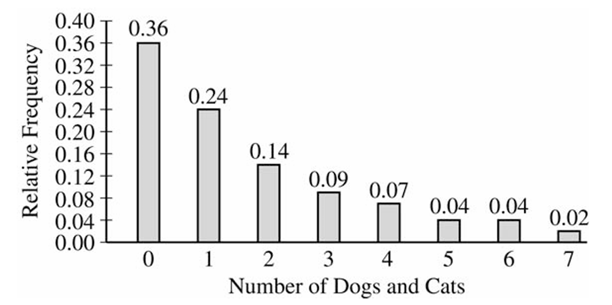
A household is in violation if it owns more than $3$ pets, i.e., $X > 3$. Read the relative frequencies for $X = 4, 5, 6, 7$ directly from the graph and add them up.
$P(X > 3) = P(X=4) + P(X=5) + P(X=6) + P(X=7)$
$P(X > 3) = 0.07 + 0.04 + 0.04 + 0.02$
$\boxed{P(X > 3) = 0.17}$

(b)
Let $Y$ = the number of households in violation among the $10$ selected. Since each household is independently either in violation or not, $Y$ follows a binomial distribution with $n = 10$ and $p = 0.17$ (from part (a)).
Using the binomial probability formula $P(Y = k) = \dbinom{n}{k} p^k (1-p)^{n-k}$:
$P(Y = 2) = \binom{10}{2}(0.17)^2(0.83)^8$
$P(Y = 2) = 45 \times (0.0289) \times (0.2252)$
$\boxed{P(Y = 2) \approx 0.2929}$

(c)
Because the sample size $n = 150$ is large, the Central Limit Theorem tells us the sampling distribution of $\bar{X}$ will be approximately normal, regardless of the shape of the original population distribution.
The mean of the sampling distribution equals the population mean:
$\mu_{\bar{X}} = \mu = 1.65$
The standard deviation (standard error) of the sampling distribution is:
$\sigma_{\bar{X}} = \dfrac{\sigma}{\sqrt{n}} = \dfrac{1.851}{\sqrt{150}} \approx 0.1511$
So the sampling distribution of $\bar{X}$ is approximately $N(1.65,\ 0.1511)$ — normal, centered at $1.65$, with a standard deviation of about $0.1511$.

Question

Golf balls must meet a set of five standards in order to be used in professional tournaments. One of these standards is distance traveled. When a ball is hit by a mechanical device, Iron Byron, with a 10-degree angle of launch, a backspin of 42 revolutions per second, and a ball velocity of 235 feet per second, the distance the ball travels may not exceed 291.2 yards. Manufacturers want to develop balls that will travel as close to the 291.2 yards as possible without exceeding that distance. A particular manufacturer has determined that the distances traveled for the balls it produces are normally distributed with a standard deviation of 2.8 yards. This manufacturer has a new process that allows it to set the mean distance the ball will travel.

(a) If the manufacturer sets the mean distance traveled to be equal to 288 yards, what is the probability that a ball that is randomly selected for testing will travel too far?

(b) Assume the mean distance traveled is 288 yards and that five balls are independently tested. What is the probability that at least one of the five balls will exceed the maximum distance of 291.2 yards?

(c) If the manufacturer wants to be 99 percent certain that a randomly selected ball will not exceed the maximum distance of 291.2 yards, what is the largest mean that can be used in the manufacturing process?

Most-appropriate topic codes (AP Statistics):

• Topic 2.11 — The Normal Distribution (Parts $\mathrm{a}$, $\mathrm{c}$)
• Topic 2.10 — The Binomial Distribution (Part $\mathrm{b}$)
• Topic 2.7 — Independent Events and Unions of Events (Part $\mathrm{b}$)

▶️ Answer/Explanation

(a)
Let $D$ represent the distance a randomly selected ball travels. We are given that $D$ is normally distributed with mean $\mu = 288$ yards and standard deviation $\sigma = 2.8$ yards.
A ball travels “too far” if it exceeds 291.2 yards, so we need:
$P(D > 291.2)$
Converting to a $z$-score:
$z = \frac{291.2 – 288}{2.8} = \frac{3.2}{2.8} = 1.14$
$P(D > 291.2) = P(Z > 1.14) = 1 – P(Z \leq 1.14) = 1 – 0.8729 = 0.1271$
$\boxed{P(D > 291.2) \approx 0.1271}$

(b)
Since five balls are independently tested and the probability that any one ball exceeds 291.2 yards is $p = 0.1271$ (from part a), the number of balls exceeding the limit follows a binomial distribution with $n = 5$ and $p = 0.1271$.
Using the complement rule:
$P(\text{at least one} > 291.2) = 1 – P(\text{none} > 291.2)$
$= 1 – P(\text{all five} \leq 291.2)$
$= 1 – (1 – 0.1271)^5$
$= 1 – (0.8729)^5$
$= 1 – 0.5068$
$= 0.4932$
$\boxed{P(\text{at least one ball exceeds 291.2 yards}) \approx 0.4932}$

(c)
We want the manufacturer to be 99 percent certain that a randomly selected ball will not exceed 291.2 yards, meaning:
$P(D \leq 291.2) = 0.99$
The 99th percentile of the standard normal distribution corresponds to $z^* = 2.33$.
Setting up the equation with the unknown mean $\mu$:
$\frac{291.2 – \mu}{2.8} = 2.33$
Solving for $\mu$:
$291.2 – \mu = 2.33 \times 2.8 = 6.524$
$\mu = 291.2 – 6.524 = 284.676$
$\boxed{\mu = 284.676 \text{ yards}}$
In order to be 99 percent certain that a randomly selected ball will not exceed the maximum distance of 291.2 yards, the largest mean that can be used in the manufacturing process is 284.676 yards.

Question

Sunshine Farms wants to know whether there is a difference in consumer preference for two new juice products — Citrus Fresh and Tropical Taste. In an initial blind taste test, 8 randomly selected consumers were given unmarked samples of the two juices. The product that each consumer tasted first was randomly decided by the flip of a coin. After tasting the two juices, each consumer was asked to choose which juice he or she preferred, and the results were recorded.

(a) Let $p$ represent the population proportion of consumers who prefer Citrus Fresh. In terms of $p$, state the hypotheses that Sunshine Farms is interested in testing.

(b) One might consider using a one-proportion $z$-test to test the hypotheses in part (a). Explain why this would not be a reasonable procedure for this sample.

(c) Let $X$ represent the number of consumers in the sample who prefer Citrus Fresh. Assuming there is no difference in consumer preference, find the probability for each possible value of $X$. Record the $x$-values and the corresponding probabilities in the table below.

(d) When testing the hypotheses in part (a), Sunshine Farms will conclude that there is a consumer preference if too many or too few individuals prefer Citrus Fresh. Based on your probabilities in part (c), is it possible for the significance level (probability of rejecting the null hypothesis when it is true) for this test to be exactly 0.05? Justify your answer.

(e) The preference data for the 8 randomly selected consumers are given in the table below.

Based on these preferences and your previous work, test the hypotheses in part (a).

(f) Sunshine Farms plans to add one of these two new juices — Citrus Fresh or Tropical Taste — to its production schedule. A follow-up study will be conducted to decide which of the two juices to produce. Make one recommendation for the follow-up study that would make it better than the initial study. Provide a statistical justification for your recommendation in the context of the problem.

Most-appropriate topic codes (AP Statistics):

• Topic 3.5 — Setting Up a Test for a Population Proportion (Part $\mathrm{a}$)
• Topic 3.2 — Sampling Distributions for Sample Proportions (Part $\mathrm{b}$)
• Topic 2.10 — The Binomial Distribution (Part $\mathrm{c}$)
• Topic 3.6 — p-Values (Part $\mathrm{d}$)
• Topic 3.7 — Carrying Out a Test for a Population Proportion (Part $\mathrm{e}$)
• Topic 1.13 — Experimental Design (Part $\mathrm{f}$)

▶️ Answer/Explanation

(a)
Let $p$ be the population proportion of consumers who prefer Citrus Fresh. The hypotheses are:
$H_0: p = 0.5$
$H_a: p \neq 0.5$
A two-sided alternative is appropriate because Sunshine Farms wants to detect any difference in preference, not just preference for one particular juice.

(b)
The conditions for a one-proportion $z$-test require that both $np$ and $n(1-p)$ be at least 5 (or 10). Here:
$np = 8 \times 0.5 = 4 < 5$
$n(1-p) = 8 \times 0.5 = 4 < 5$
Since both values are less than 5, the large-sample normal approximation is not valid, and using a one-proportion $z$-test would not be appropriate for a sample of only $n = 8$.

(c)
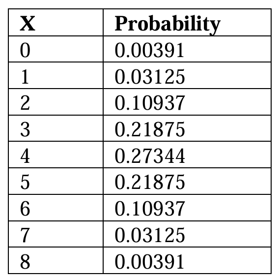
Under $H_0$, $X \sim \text{Binomial}(n = 8,\ p = 0.5)$. The probabilities are computed using:
$P(X = x) = \binom{8}{x}(0.5)^x(0.5)^{8-x} = \binom{8}{x}(0.5)^8$

(d)
No, it is not possible for the significance level to be exactly 0.05. Because $X$ is a discrete random variable, the tail probabilities can only take specific values — there is no rejection region that gives a type I error probability of exactly 0.05.
The most extreme rejection region $(X = 0 \text{ or } X = 8)$ gives:
$\alpha = 2 \times 0.00391 = 0.00782 < 0.05$
The next possible rejection region $(X \leq 1 \text{ or } X \geq 7)$ gives:
$\alpha = 2 \times (0.00391 + 0.03125) = 2 \times 0.03516 = 0.07031 > 0.05$
Since no rejection region produces a type I error probability of exactly 0.05, a significance level of exactly 0.05 is not achievable with this test.
$\boxed{\alpha = 0.05 \text{ is not achievable — the achievable levels jump from } 0.00782 \text{ to } 0.07031}$

(e)
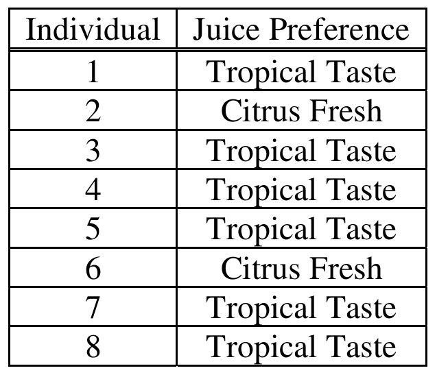
From the data, 2 out of 8 consumers preferred Citrus Fresh, so $X = 2$.
Since this is a two-sided test, the $p$-value is the probability of observing a result at least as extreme as $X = 2$ in either tail:
$p\text{-value} = P(X \leq 2) + P(X \geq 6)$
$= 2 \times [P(X=0) + P(X=1) + P(X=2)]$
$= 2 \times (0.00391 + 0.03125 + 0.10937)$
$= 2 \times 0.14453 = 0.28906$
Since the $p$-value of $0.289$ is much larger than any reasonable significance level (e.g., $\alpha = 0.05$ or $\alpha = 0.07031$), we fail to reject $H_0$. There is not statistically significant evidence of a consumer preference between Citrus Fresh and Tropical Taste.
$\boxed{p\text{-value} \approx 0.289 \implies \text{Fail to reject } H_0; \text{ no significant consumer preference detected}}$

(f)
The most important recommendation is to increase the number of consumers in the study. With only $n = 8$ consumers, the test has very low power — even a large true difference in preference (like 75% vs. 25%) may not produce a statistically significant result. Increasing the sample size would reduce the standard error of the estimated proportion $\hat{p}$, making it easier to detect a real difference, and would allow the use of the large-sample one-proportion $z$-test since $np \geq 5$ and $n(1-p) \geq 5$ would be satisfied. For example, with $n = 80$ and $X = 20$ (same sample proportion of 0.25), the $z$-statistic would be approximately:
$z = \frac{0.25 – 0.5}{\sqrt{\frac{0.5(0.5)}{80}}} \approx -4.47$
which gives a $p$-value near zero, allowing a clear conclusion to be reached.
$\boxed{\text{Recommendation: Increase sample size to increase power and enable use of the } z\text{-test}}$

Question

At an archaeological site that was an ancient swamp, the bones from 20 brontosaur skeletons have been unearthed. The bones do not show any sign of disease or malformation. It is thought that these animals wandered into a deep area of the swamp and became trapped in the swamp bottom. The 20 left femur bones (thigh bones) were located and 4 of these left femurs are to be randomly selected without replacement for DNA testing to determine gender.

(a) Let $X$ be the number out of the 4 selected left femurs that are from males. Based on how these bones were sampled, explain why the probability distribution of $X$ is not binomial.

(b) Suppose that the group of 20 brontosaurs whose remains were found in the swamp had been made up of 10 males and 10 females. What is the probability that all 4 in the sample to be tested are male?

(c) The DNA testing revealed that all 4 femurs tested were from males. Based on this result and your answer from part (b), do you think that males and females were equally represented in the group of 20 brontosaurs stuck in the swamp? Explain.

(d) Is it reasonable to generalize your conclusion in part (c) pertaining to the group of 20 brontosaurs to the population of all brontosaurs? Explain why or why not.

Most-appropriate topic codes (AP Statistics):

• Topic 2.10 — The Binomial Distribution (Part a)
• Topic 2.7 — Independent Events and Unions of Events (Part a,b)
• Topic 2.4 — Introduction to Probability (Part b)
• Topic 2.3 — Estimating Probabilities Using Simulation (Part c)
•Topic 1.12 — Potential Problems with Sampling (Part d)

▶️ Answer/Explanation

(a)
The probability distribution of $X$ is not binomial because the bones are selected without replacement from a finite population of only 20 femurs. For a binomial distribution to apply, each trial must be independent — that is, the probability of success (selecting a male femur) must remain constant from one draw to the next. However, when sampling without replacement, the composition of the remaining pool changes with each selection, so the probability of drawing a male femur on each successive draw depends on what was drawn before it. Since the trials are not independent and the probability of success is not fixed, the distribution of $X$ is hypergeometric, not binomial.
$\boxed{X \text{ is not binomial because sampling is without replacement, making trials dependent}}$

(b)
With 10 males and 10 females among the 20 brontosaurs, compute the probability that all 4 selected femurs are male using the multiplication rule for dependent events (without replacement):
$P(\text{1st is male}) = \dfrac{10}{20}$
$P(\text{2nd is male} \mid \text{1st is male}) = \dfrac{9}{19}$
$P(\text{3rd is male} \mid \text{first two are male}) = \dfrac{8}{18}$
$P(\text{4th is male} \mid \text{first three are male}) = \dfrac{7}{17}$
Therefore:
$P(\text{all 4 are male}) = \dfrac{10}{20} \times \dfrac{9}{19} \times \dfrac{8}{18} \times \dfrac{7}{17}$
$= \dfrac{10 \times 9 \times 8 \times 7}{20 \times 19 \times 18 \times 17} = \dfrac{5040}{116280} \approx 0.0433$
This can also be expressed using combinations:
$P(\text{all 4 are male}) = \dfrac{\dbinom{10}{4}}{\dbinom{20}{4}} = \dfrac{210}{4845} \approx 0.0433$
$\boxed{P(\text{all 4 male}) \approx 0.0433}$

(c)
No, it does not seem likely that males and females were equally represented in the group of 20 brontosaurs. From part (b), if the group had exactly 10 males and 10 females, the probability of randomly selecting 4 males in a row is only about $4.33\%$. Since this probability is quite small (less than 5%), observing all 4 selected femurs being male is an unusual result under the assumption of equal representation. It is therefore more reasonable to think that males outnumbered females in this particular group of brontosaurs trapped in the swamp, though equal representation is possible — just unlikely given the data.
$\boxed{\text{Equal representation is unlikely; evidence suggests more males than females in the group}}$

(d)
No, it is not reasonable to generalize the conclusion from part (c) to the entire population of brontosaurs. The 20 brontosaurs found at the site do not constitute a random sample from the population of all brontosaurs — they represent only those individuals that happened to wander into that particular swamp and become trapped. This is a highly specific and non-random group. It is plausible that behavioral differences between male and female brontosaurs (for example, males may have been more likely to venture into deep swamp areas while foraging) could explain why males are overrepresented in this particular site. Such a non-representative sample cannot be used to draw conclusions about the broader population of all brontosaurs.
$\boxed{\text{Cannot generalize; the 20 brontosaurs are not a random sample of all brontosaurs}}$

Question

Men’s shirt sizes are determined by their neck sizes. Suppose that men’s neck sizes are approximately normally distributed with mean $15.7$ inches and standard deviation $0.7$ inch. A retailer sells men’s shirts in sizes S, M, L, XL, where the shirt sizes are defined in the table below.

(a) Because the retailer only stocks the sizes listed above, what proportion of customers will find that the retailer does not carry any shirts in their sizes? Show your work.

(b) Using a sketch of a normal curve, illustrate the proportion of men whose shirt size is M. Calculate this proportion.

(c) Of $12$ randomly selected customers, what is the probability that exactly $4$ will request size M? Show your work.

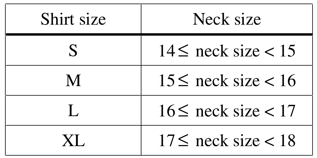
Most-appropriate topic codes (AP Statistics):

• Topic 2.11 — The Normal Distribution (Parts a, b)
• Topic 2.10 — The Binomial Distribution (Part c)

▶️ Answer/Explanation

(a)
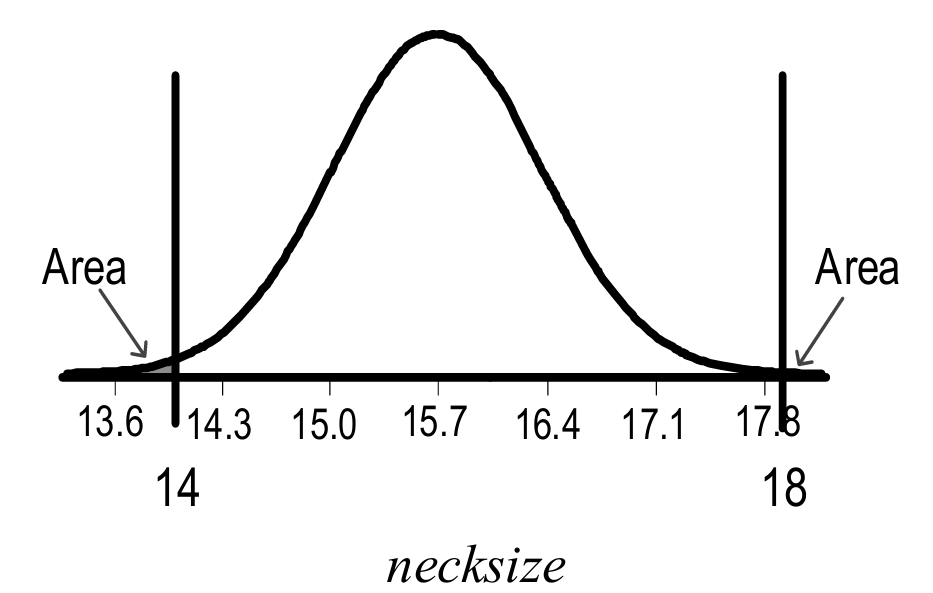
A customer “misses out” if their neck size falls outside the range covered by S through XL, that is, below $14$ inches or at $18$ inches or above. So we need two tail probabilities:
$ P(\text{neck size}<14 \text{ or } \text{neck size}\ge18)=P(\text{neck size}<14)+P(\text{neck size}\ge18) $
Convert each cutoff to a $z$-score using $z=\dfrac{x-\mu}{\sigma}$:
$ z_1=\dfrac{14-15.7}{0.7}\approx-2.43 $
$ z_2=\dfrac{18-15.7}{0.7}\approx3.29 $
From the standard normal table:
$ P(z<-2.43)\approx0.0076 $
$ P(z>3.29)\approx0.0005 $
Adding these two tail areas together:
$ 0.0076+0.0005\approx0.0081 $
$ \boxed{\text{About } 0.81\% \text{ of customers will not find their size.}} $

(b)
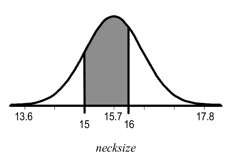
Size M corresponds to neck sizes from $15$ up to (but not including) $16$ inches, so we need the area under the normal curve between these two values.

Convert both boundaries to $z$-scores:
$ z_1=\dfrac{15-15.7}{0.7}=-1.00 $
$ z_2=\dfrac{16-15.7}{0.7}\approx0.43 $
The proportion is the area between these two $z$-values:
$ P(-1.00<z<0.43)=P(z<0.43)-P(z<-1.00) $
$ P(-1.00<z<0.43)\approx0.6664-0.1587 $
$ P(-1.00<z<0.43)\approx0.5077 $
$ \boxed{\text{About } 50.77\% \text{ of men wear size M.}} $

(c)
Each of the $12$ customers independently either requests size M or doesn’t, with the same probability of “success” each time — that’s a binomial setting. Let $X$ be the number of customers (out of $12$) who request size M.
$ X\sim\text{Binomial}(n=12,\ p=0.5077) $
We want the probability of exactly $4$ successes, so we use the binomial formula:
$ P(X=4)=\binom{12}{4}(0.5077)^4(0.4923)^8 $
Work out each piece separately. The number of ways to choose which $4$ of the $12$ customers want size M:
$ \binom{12}{4}=495 $
The probability that $4$ specific customers all want M:
$ (0.5077)^4\approx0.0664 $
The probability that the remaining $8$ customers all want something else:
$ (0.4923)^8\approx0.00347 $
Multiply everything together:
$ P(X=4)\approx495\times0.0664\times0.00347 $
$ P(X=4)\approx0.1139 $
$ \boxed{P(X=4)\approx0.1139} $

AP Statistics 2.10 The Binomial Distribution- Exam Style Questions - FRQs - New Syllabus

Question

Question

Question

Question

Question

Question

Question

Question

Question

Question

Question

Question

Question

Question

Resources

Members

Company