
AP Statistics 2.11 The Normal Distribution- Exam Style Questions - FRQs - New Syllabus
Question
(ii) Suppose Cleo took a random sample of $n=2$ necklaces that resulted in a sample mean amount of gold applied of 303 mg. Would that result indicate that the population mean amount of gold being applied by the machine is different from 300 mg? Justify your answer without performing an inference procedure.
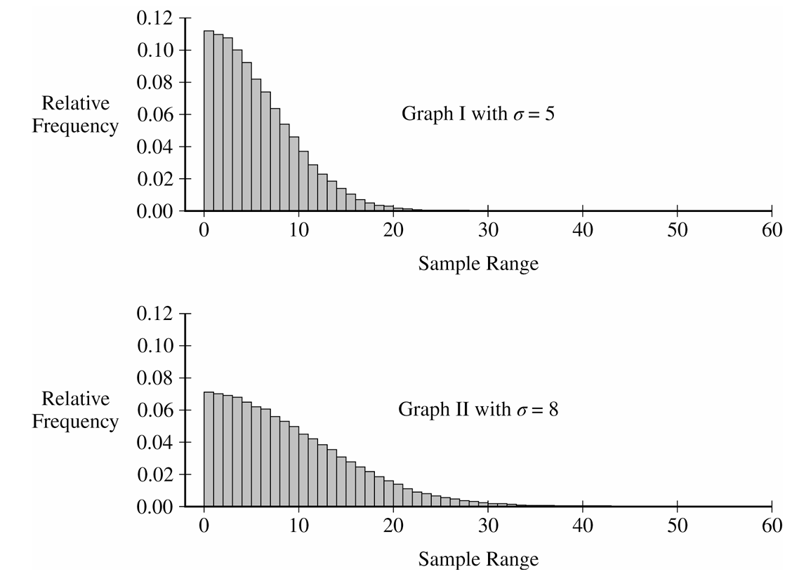
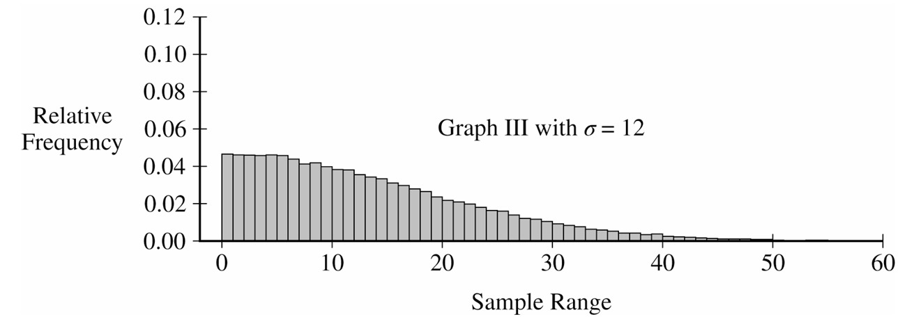
(ii) Describe how the sampling distribution of the sample range for samples of size $n=2$ changes as the value of the population standard deviation increases.
(ii) Do Cleo’s sample mean of 303 mg and range of 10 mg indicate that the machine is not working properly? Explain your answer.
Most-appropriate topic codes (AP Statistics):
• Topic \(2.11\) — The Normal Distribution (Part \( \mathrm{a} \))
• Topic \(2.12\) — Central Limit Theorem and Sampling Distributions for Sample Means (Parts \( \mathrm{b} \), \( \mathrm{d} \))
▶️ Answer/Explanation
(a)
To find the probability, standardize the given values to z-scores using the formula $z = \frac{x – \mu}{\sigma}$.
$P(296 < X < 304) = P\left(\frac{296-300}{5} < Z < \frac{304-300}{5}\right)$
This simplifies to $P(-0.8 < Z < 0.8) \approx 0.5762$.
(b) (i)
For $n=2$, the standard error of the mean is $\sigma_{\bar{x}} = \frac{5}{\sqrt{2}} \approx 3.535$.
$P(\bar{X} > 303) = P\left(Z > \frac{303-300}{3.535}\right) = P(Z > 0.849)$
$P(\bar{X} > 303) \approx 0.198$.
(b) (ii)
No, this result would not indicate the machine is malfunctioning. Because a sample mean of $303$ mg or higher has a probability of approximately $0.198$ (about $20\%$) assuming the machine is working properly, this result is fairly common and not unusual.
(c) (i)
The sampling distribution of the sample range is heavily right-skewed. The center is around a sample range of $4$ to $5$ mg, and the values vary from $0$ mg up to approximately $25$ mg.
(c) (ii)
As the population standard deviation increases, the center of the sampling distribution shifts to the right (indicating a larger expected range), and the distribution becomes more spread out, showing greater variability in the possible sample ranges.
(d) (i)
No, a sample range of $10$ mg is not unusual. Looking at Graph I (where $\sigma=5$), the bars at and to the right of $10$ mg make up a substantial portion of the total area (well over $5\%$), meaning a range of $10$ mg or more occurs quite frequently by chance.
(d) (ii)
No, these results do not indicate a problem. Based on part (b), a sample mean of $303$ mg is not unusual (happens about $20\%$ of the time), and based on part (d)(i), a sample range of $10$ mg is also quite typical. Since neither metric is statistically surprising, there is no convincing evidence to doubt the machine is working properly.
Question
(ii) Determine the probability that a crate will be rejected by the warehouse manager. Show your work.
Most-appropriate topic codes (AP Statistics):
• Topic \(2.11\) — The Normal Distribution (Parts \( \mathrm{a} \), \( \mathrm{c} \))
▶️ Answer/Explanation
(a)
Let $A$ be the amount of shampoo in a bottle. We need to find $P(A < 0.50)$.
$z = \frac{0.50 – 0.60}{0.04} = -2.5$
$P(A < 0.50) = P(Z < -2.5) = 0.0062$
(b)(i)
Let $X$ represent the number of underfilled bottles in a randomly selected box of 10 bottles. Because each bottle’s volume is independent and has the same probability of being underfilled, the random variable $X$ has a binomial distribution with $n = 10$ trials and probability of success $p = 0.0062$.
(b)(ii)
The probability that a crate will be rejected is the probability of finding 2 or more underfilled bottles in a box: $P(X \ge 2)$.
$P(X \ge 2) = 1 – P(X \le 1) = 1 – [P(X = 0) + P(X = 1)]$
$P(X \ge 2) = 1 – \left[\binom{10}{0}(0.0062)^0(0.9938)^{10} + \binom{10}{1}(0.0062)^1(0.9938)^9\right]$
$P(X \ge 2) \approx 1 – [0.9397 + 0.0586] \approx 1 – 0.9983 = 0.0017$
(c)
Under the adjusted programming, the new mean is $0.56$ and the standard deviation is $0.03$. The new probability of a bottle being underfilled is:
$z = \frac{0.50 – 0.56}{0.03} = -2.0$
$P(Z < -2.0) \approx 0.02275$
Because the probability of an underfilled bottle is much greater for the adjusted programming ($0.0228$) than for the original programming ($0.0062$), the manufacturing company should keep the original programming. Using the adjusted settings would actually result in more underfilled bottles, thereby increasing the number of rejected crates.
Question
Most-appropriate topic codes (AP Statistics):
• Topic \(2.9\) — Parameters of Random Variables (Part \( \mathrm{c} \))
• Topic \(2.11\) — The Normal Distribution (Parts \( \mathrm{a} \), \( \mathrm{b} \))
▶️ Answer/Explanation
(a)
We need to find the \(25\text{th}\) percentile of the normal distribution.
Looking at the standard normal distribution table, the \(z\)-score that corresponds to a left-tail area of \(0.25\) is approximately \(-0.6745\).
We can set up the formula for the \(z\)-score and solve for \(x\):
\(z = \dfrac{x – \mu}{\sigma}\)
\(-0.6745 = \dfrac{x – 30}{8}\)
\(x = 30 + 8(-0.6745) \approx 24.6\)
It is expected that \(25\) percent of the batteries will no longer work after approximately \(24.6\) months.
(b)
We are looking for the probability that the battery lifespan is less than \(24\) months.
First, we calculate the \(z\)-score for \(x = 24\):
\(z = \dfrac{24 – 30}{8}\)
\(z = -0.75\)
Using the standard normal probability table, the probability \(P(Z < -0.75)\) is roughly \(0.2266\).
The probability that the customer will require a replacement is \(0.2266\).
(c)
Let \(X\) represent the company’s financial gain per warranty purchased.
The probability that a replacement is required is \(0.2266\), resulting in a loss of \(\$150\).
The probability that a replacement is NOT required is \(1 – 0.2266 = 0.7734\), resulting in a gain of \(\$50\).
The expected value \(E(X)\) is the sum of each outcome multiplied by its corresponding probability:
\(E(X) = (50)(0.7734) + (-150)(0.2266)\)
\(E(X) = 38.67 – 33.99\)
\(E(X) = \$4.68\)
The expected gain for the company per warranty purchased is \(\$4.68\).
Question
Most-appropriate topic codes (AP Statistics):
• Topic \(2.7\) — Independent Events and Mutually Exclusive Events (Parts \( \mathrm{b} \), \( \mathrm{c} \))
• Topic \(2.11\) — The Normal Distribution (Part \( \mathrm{a} \))
▶️ Answer/Explanation
(a)
Let \(X\) denote the diameter (in mm) of a randomly selected melon from Distributor J. We are told that \(X\) follows an approximately normal distribution with mean \(\mu = 133\) mm and standard deviation \(\sigma = 5\) mm.
First, convert the boundary value to a \(z\)-score:
\( z = \dfrac{137 – 133}{5} = \dfrac{4}{5} = 0.8 \)
Now find the probability to the right of \(z = 0.8\) using the standard normal table:
\( P(X > 137) = P(Z > 0.8) = 1 – P(Z < 0.8) = 1 – 0.7881 \)
\( \boxed{P(X > 137) = 0.2119} \)
(b)
Define the following events:
\(J\): the melon is from Distributor J
\(K\): the melon is from Distributor K
\(G\): the melon has a diameter greater than \(137\) mm
We are given \(P(J) = 0.70\), \(P(K) = 0.30\), \(P(G \mid J) = 0.2119\), and \(P(G \mid K) = 0.8413\).
Using the Law of Total Probability:
\( P(G) = P(G \mid J)\cdot P(J) + P(G \mid K)\cdot P(K) \)
\( P(G) = (0.2119)(0.70) + (0.8413)(0.30) \)
\( P(G) = 0.14833 + 0.25239 \)
\( \boxed{P(G) = 0.4007} \)
(c)
We want the conditional probability that the melon is from Distributor J, given that its diameter is greater than \(137\) mm. Using the definition of conditional probability:
\( P(J \mid G) = \dfrac{P(J \cap G)}{P(G)} \)
The joint probability \(P(J \cap G)\) was found in part (b):
\( P(J \cap G) = P(G \mid J)\cdot P(J) = (0.2119)(0.70) = 0.14833 \)
Substituting into the formula:
\( P(J \mid G) = \dfrac{0.14833}{0.40072} \)
\( \boxed{P(J \mid G) \approx 0.3701} \)
Even though Distributor J supplies \(70\%\) of the melons in the store, only about \(37\%\) of the large-diameter melons (over \(137\) mm) come from Distributor J — this makes sense because Distributor K’s melons are much more likely to be large, so they dominate that group despite being the smaller supplier.
Question
Most-appropriate topic codes (AP Statistics):
• Topic \(2.9\) — Parameters of Random Variables (Part \( \mathrm{b}\text{-}\mathrm{i} \), Part \( \mathrm{b}\text{-}\mathrm{ii} \))
▶️ Answer/Explanation
(a)
Let \(W\) denote the weight of a randomly selected full carton. Then \(W \sim N(840,\ 7.9)\).
Compute the \(z\)-score for \(850\) grams:
$z = \frac{850 – 840}{7.9} \approx 1.27$
Using the standard normal table:
$P(W > 850) = P(Z > 1.27) = 1 – 0.8980$
$\boxed{P(W > 850) \approx 0.1020}$
(b)(i)
Let \(P\) be the weight of the empty cardboard container and \(X_1, X_2, \ldots, X_{12}\) be the weights of the \(12\) eggs. Then the weight of a full carton is:
$W = P + X_1 + X_2 + \cdots + X_{12}$
Taking expected values of both sides:
$E(W) = E(P) + 12\,E(X)$
Substituting the known values \(E(W) = 840\) and \(E(P) = 20\):
$840 = 20 + 12\,E(X)$
$E(X) = \frac{840 – 20}{12} = \frac{820}{12}$
$\boxed{\mu_X \approx 68.33 \text{ grams}}$
(b)(ii)
Since all variables are independent, variances add:
$\text{Var}(W) = \text{Var}(P) + 12\,\text{Var}(X)$
We know \(\text{Var}(W) = (7.9)^2 = 62.41\) and \(\text{Var}(P) = (1.7)^2 = 2.89\). Substituting:
$62.41 = 2.89 + 12\,\text{Var}(X)$
$\text{Var}(X) = \frac{62.41 – 2.89}{12} = \frac{59.52}{12} = 4.96$
$\sigma_X = \sqrt{4.96}$
$\boxed{\sigma_X \approx 2.23 \text{ grams}}$
Question


Most-appropriate topic codes (AP Statistics):
• Topic 1.7 — Summary Statistics for One Quantitative Variable (Part b)
• Topic 1.9 — Comparisons of the Distributions for One Quantitative Variable (Part c)
▶️ Answer/Explanation
(a)
No, it is not reasonable to believe that the distribution of running times is approximately normal.
In a normal distribution, data extends several standard deviations below the mean. For this dataset, the minimum running time is \(4.40\) seconds, which yields a standardized distance from the mean of:
\(z = \dfrac{4.40 – 4.60}{0.15} = -1.33\)
Since a normal distribution expects approximately \(9.2\%\) of its observations to fall below \(1.33\) standard deviations beneath the mean, having a hard cutoff at \(1.33\) standard deviations indicates that the left tail is severely truncated. Thus, the distribution is likely skewed to the right.
(b)
To find the standardized score for a weight of \(370\) pounds, we use the z-score formula:
\(z = \dfrac{x – \mu}{\sigma}\)
\(z = \dfrac{370 – 310}{25} = \dfrac{60}{25} = 2.40\)
Interpretation: This player’s weightlifting performance is \(2.40\) standard deviations above the average weight lifted by all players in this position.
(c)
The team should select Player A.
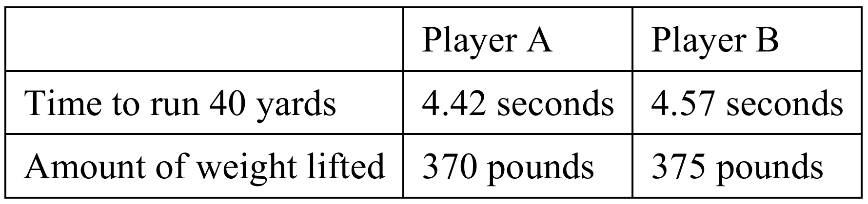
To perform a fair comparison since both speed and strength carry equal importance, we compute the z-scores for both players on each metric:
Player A:
\(z_{\text{speed}} = \dfrac{4.42 – 4.60}{0.15} = -1.20\)
\(z_{\text{strength}} = \dfrac{370 – 310}{25} = 2.40\)
Since a lower running time indicates a more desirable speed, a negative z-score is a positive attribute. The combined standardized advantage for Player A is \(2.40 – (-1.20) = 3.60\) units of desirability (or we can think of a speed index where faster is positive, meaning a net sum of \(1.20 + 2.40 = 3.60\)).
Player B:
\(z_{\text{speed}} = \dfrac{4.57 – 4.60}{0.15} = -0.20\)
\(z_{\text{strength}} = \dfrac{375 – 310}{25} = 2.60\)
The combined standardized index advantage for Player B is \(0.20 + 2.60 = 2.80\).
Comparing the two candidates, Player A is dramatically faster than Player B (\(1.20\) standard deviations below the mean versus only \(0.20\) standard deviations below), while Player B is only slightly stronger than Player A (\(2.60\) standard deviations above the mean versus \(2.40\)). Therefore, Player A represents a significantly better overall draft value when both metrics are weighted equally.
Question
Most-appropriate topic codes (AP Statistics):
• Topic \(2.10\) — The Binomial Distribution (Part \(\mathrm{b}\))
• Topic \(2.12\) — Sampling Distributions and the Central Limit Theorem (Part \(\mathrm{c}\))
▶️ Answer/Explanation
(a)
Let \(X\) denote the stopping distance. We are told that \(X\) is normally distributed with
\( \mu_X = 125 \text{ ft}, \qquad \sigma_X = 6.5 \text{ ft} \)
We want the value \(x\) such that \(P(X \leq x) = 0.70\).
From the standard normal table, the \(z\)-score with a cumulative probability of \(0.70\) is
\( z = 0.52 \)
Using the \(z\)-score formula and solving for \(x\):
\( z = \dfrac{x – \mu}{\sigma} \implies x = \mu + z\sigma \)
\( x = 125 + 0.52(6.5) = 125 + 3.38 \)
\( \boxed{x \approx 128.4 \text{ feet}} \)
So the 70th percentile of the stopping distance distribution is approximately \(128.4\) feet — meaning \(70\%\) of cars stop within this distance.
(b)
From part (a), a stopping distance greater than \(128.4\) feet corresponds to the top \(30\%\) of the distribution:
\( p = P(X > 128.4) = 1 – 0.70 = 0.30 \)
Let \(Y\) = number of cars (out of 5) that stop in a distance greater than \(128.4\) feet. Since each car is independent and the probability of “success” is the same for each, \(Y\) follows a binomial distribution:
\( Y \sim B(n=5,\ p=0.30) \)
We need \(P(Y \geq 2)\). It is easier to use the complement:
\( P(Y \geq 2) = 1 – P(Y \leq 1) = 1 – \bigl[P(Y=0) + P(Y=1)\bigr] \)
\( P(Y=0) = \binom{5}{0}(0.30)^0(0.70)^5 = 1 \cdot 1 \cdot 0.16807 = 0.16807 \)
\( P(Y=1) = \binom{5}{1}(0.30)^1(0.70)^4 = 5 \cdot 0.30 \cdot 0.2401 = 0.36015 \)
\( P(Y \leq 1) = 0.16807 + 0.36015 = 0.52822 \)
\( P(Y \geq 2) = 1 – 0.52822 \)
\( \boxed{P(Y \geq 2) \approx 0.4718} \)
There is roughly a \(47.18\%\) chance that at least 2 of the 5 randomly selected cars will stop beyond \(128.4\) feet — think of it as just under a coin-flip, which makes intuitive sense since each car has a \(30\%\) chance on its own.
(c)
Let \(\bar{X}\) denote the mean stopping distance of a random sample of \(n = 5\) cars. Because the individual stopping distances are normally distributed, the sampling distribution of \(\bar{X}\) is also exactly normal with:
\( \mu_{\bar{X}} = \mu = 125 \text{ ft} \)
\( \sigma_{\bar{X}} = \dfrac{\sigma}{\sqrt{n}} = \dfrac{6.5}{\sqrt{5}} \approx 2.907 \text{ ft} \)
We want \(P(\bar{X} \geq 130)\). Convert to a \(z\)-score:
\( z = \dfrac{130 – 125}{6.5/\sqrt{5}} = \dfrac{5}{2.907} \approx 1.72 \)
\( P(\bar{X} \geq 130) = P(Z \geq 1.72) = 1 – P(Z < 1.72) \)
\( P(Z < 1.72) \approx 0.9573 \)
\( P(\bar{X} \geq 130) = 1 – 0.9573 \)
\( \boxed{P(\bar{X} \geq 130) \approx 0.0427} \)
There is only about a \(4.27\%\) chance that the average stopping distance for 5 randomly selected cars exceeds 130 feet — this is much smaller than the \(30\%\) chance for any single car, because averaging over 5 cars reduces variability considerably and makes extreme means much less likely.
Question
Most-appropriate topic codes (AP Statistics):
• Topic 2.9 — Parameters of Random Variables (Part \(\mathrm{a}\))
• Topic 2.11 — The Normal Distribution (Parts \(\mathrm{b}\), \(\mathrm{c}\))
▶️ Answer/Explanation
(a)
Since \(X\) and \(Y\) are independent normal random variables, their difference \(Y – X\) is also normally distributed. The mean and standard deviation of \(Y – X\) are found as follows:
\(\mu_{Y-X} = \mu_Y – \mu_X = 200 – 170 = 30 \text{ minutes}\)
\(\sigma_{Y-X} = \sqrt{\sigma_Y^2 + \sigma_X^2} = \sqrt{10^2 + 20^2} = \sqrt{100 + 400} = \sqrt{500} \approx 22.36 \text{ minutes}\)
\(\boxed{Y – X \sim N(30,\ 22.36^2)}\)
The distribution of \(Y – X\) is normal with mean \(30\) minutes and standard deviation \(22.36\) minutes (variance \(500\)).
(b)
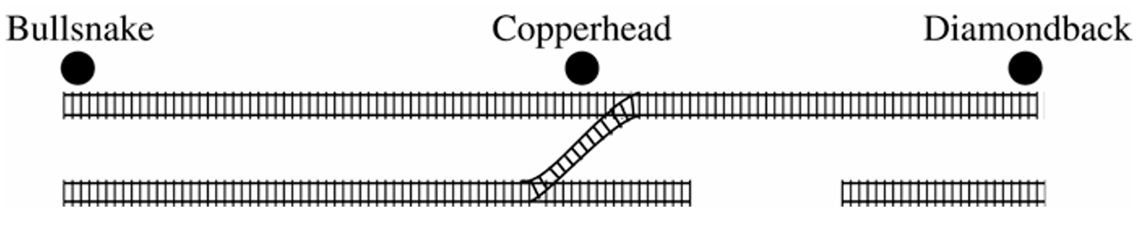
The train from Bullsnake has to wait when it arrives at Copperhead before the train from Diamondback — that is, when \(X < Y\), or equivalently when \(Y – X > 0\).
Standardize to find the \(z\)-score:
\(z = \dfrac{0 – 30}{22.36} = \dfrac{-30}{22.36} \approx -1.34\)
So the required probability is:
\(P(Y – X > 0) = P\!\left(z > -1.34\right) = 1 – P(z < -1.34) = 1 – 0.0901 = 0.9099\)
\(\boxed{P(\text{wait}) \approx 0.91}\)
About \(91\%\) of days the train from Bullsnake will have to wait at Copperhead.
(c)
Let \(D\) be the delay (in minutes) added to the Bullsnake train’s departure. The new travel-plus-delay time for the Bullsnake train is \(X + D\), where \(D\) is a constant. The difference \(Y – (X + D)\) is then normally distributed with:
\(\mu_{Y-(X+D)} = 200 – (170 + D) = 30 – D\)
\(\sigma_{Y-(X+D)} = 22.36 \text{ (unchanged, since } D \text{ is constant)}\)
We want \(P\!\left(Y – (X+D) > 0\right) = 0.01\). This means the right-tail area above \(0\) equals \(0.01\), so the left-tail area below \(0\) equals \(0.99\). The corresponding \(z\)-score for \(0.99\) is \(z = 2.33\).
Setting up the equation:
\(z = \dfrac{0 – (30 – D)}{22.36} = 2.33\)
\(0 – (30 – D) = 2.33 \times 22.36\)
\(D – 30 = 52.10\)
\(D = 82.10 \text{ minutes}\)
\(\boxed{D \approx 82 \text{ minutes}}\)
The Snake Gulch Railroad should delay the departure of the train from Bullsnake by approximately \(82\) minutes so that the probability of having to wait drops to only \(0.01\).
Question
Most-appropriate topic codes (AP Statistics):
• Topic 4.1 — Sampling Distributions for Sample Means (Part \(\mathrm{a}\))
• Topic 2.11 — The Normal Distribution (Part \(\mathrm{b}\))
▶️ Answer/Explanation
(a)
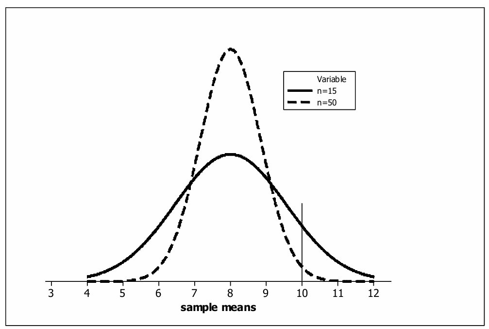
A random sample of \(n = 15\) fish is more likely to have a sample mean greater than 10 inches.
Both sampling distributions are centered at the true mean \(\mu = 8\) inches, but they differ in their variability. The standard deviation of the sampling distribution of the sample mean is given by \(\dfrac{\sigma}{\sqrt{n}}\), so a smaller sample size produces a larger standard deviation — meaning the distribution is more spread out.
Since the sampling distribution for \(n = 15\) is more spread out than for \(n = 50\), the tail area beyond 10 inches is larger for \(n = 15\), making it more likely to observe a sample mean greater than 10 inches with the smaller sample.
\(\boxed{P(\bar{x} > 10 \mid n=15) > P(\bar{x} > 10 \mid n=50) \text{ because the } n=15 \text{ distribution has greater variability.}}\)
(b)
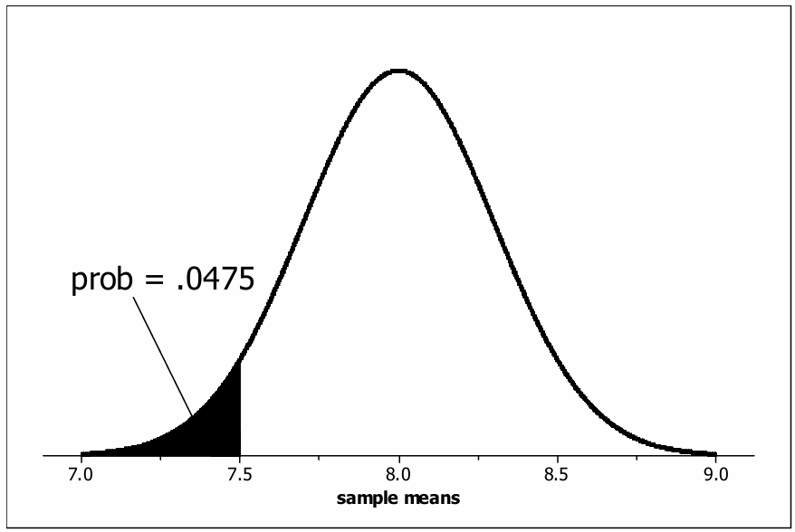
We are given: \(\mu = 8\), \(\sigma_{\bar{x}} = 0.3\), and we want \(P(\bar{x} < 7.5)\).
First, compute the \(z\)-score:
\(z = \dfrac{\bar{x} – \mu}{\sigma_{\bar{x}}} = \dfrac{7.5 – 8}{0.3} = \dfrac{-0.5}{0.3} \approx -1.67\)
Now look up the standard normal table for \(z = -1.67\):
\(P(\bar{x} < 7.5) = P(z < -1.67) \approx 0.0475\)
\(\boxed{P(\bar{x} < 7.5) \approx 0.0475}\)
(c)
Yes, it would still be appropriate to use the normal distribution to compute this probability.
By the Central Limit Theorem (CLT), the sampling distribution of the sample mean \(\bar{x}\) is approximately normal for sufficiently large sample sizes, regardless of the shape of the population distribution.
Since our sample size is \(n = 50\), which is reasonably large (generally \(n \geq 30\) is considered sufficient), the CLT guarantees that \(\bar{x}\) follows an approximately normal distribution even if the individual fish lengths are nonnormally distributed.
Therefore, the probability calculated in part (b) remains a good approximation.
\(\boxed{\text{Yes — by the CLT, } n = 50 \text{ is large enough for the sampling distribution of } \bar{x} \text{ to be approximately normal.}}\)
Question
Most-appropriate topic codes (AP Statistics):
• Topic 2.7 — Independent Events and Unions of Events (Part \(\mathrm{b}\))
• Topic 2.12 — Sampling Distributions and the Central Limit Theorem (Part \(\mathrm{c}\))
▶️ Answer/Explanation
(a)
Since \(M = D + E\) is a normal random variable plus a constant, \(M\) is also normally distributed.
With true depth \(D = 2\) feet, the distribution of \(M\) has:
\(\mu_M = 2\,\text{feet}, \qquad \sigma_M = 1.5\,\text{feet}\)
We want \(P(M < 0)\). Standardizing:
\(P(M < 0) = P\!\left(Z < \frac{0 – 2}{1.5}\right) = P(Z < -1.33)\)
Using the standard normal table:
\(\boxed{P(M < 0) \approx 0.0918}\)
(b)
Let each individual measurement be negative with probability \(p = 0.0918\) (from part (a)), and let the three measurements be independent.
Using the complement rule — it is easier to find the probability that none of the three measurements is negative, then subtract from 1:
\(P(\text{at least one negative}) = 1 – P(\text{none negative})\)
\(= 1 – (1 – 0.0918)^3\)
\(= 1 – (0.9082)^3\)
\(= 1 – 0.7491\)
\(\boxed{P(\text{at least one negative}) \approx 0.2509}\)
(c)
Let \(\bar{X}\) denote the mean of three independent depth measurements where the true depth is \(2\) feet.
Since each measurement is normally distributed, the sampling distribution of \(\bar{X}\) is also normal with:
\(\mu_{\bar{X}} = 2\,\text{feet}, \qquad \sigma_{\bar{X}} = \frac{1.5}{\sqrt{3}} = 0.8660\,\text{feet}\)
We want \(P(\bar{X} < 0)\). Standardizing:
\(P(\bar{X} < 0) = P\!\left(Z < \frac{0 – 2}{1.5/\sqrt{3}}\right) = P\!\left(Z < \frac{-2}{0.8660}\right) = P(Z < -2.31)\)
Using the standard normal table:
\(\boxed{P(\bar{X} < 0) \approx 0.0104}\)
Question
Most-appropriate topic codes (AP Statistics):
• Topic 2.10 — The Binomial Distribution (Part \(\mathrm{b}\))
• Topic 2.7 — Independent Events and Unions of Events (Part \(\mathrm{b}\))
▶️ Answer/Explanation
(a)
Let \(D\) represent the distance a randomly selected ball travels. We are given that \(D\) is normally distributed with mean \(\mu = 288\) yards and standard deviation \(\sigma = 2.8\) yards.
A ball travels “too far” if it exceeds 291.2 yards, so we need:
\(P(D > 291.2)\)
Converting to a \(z\)-score:
\(z = \frac{291.2 – 288}{2.8} = \frac{3.2}{2.8} = 1.14\)
\(P(D > 291.2) = P(Z > 1.14) = 1 – P(Z \leq 1.14) = 1 – 0.8729 = 0.1271\)
\(\boxed{P(D > 291.2) \approx 0.1271}\)
(b)
Since five balls are independently tested and the probability that any one ball exceeds 291.2 yards is \(p = 0.1271\) (from part a), the number of balls exceeding the limit follows a binomial distribution with \(n = 5\) and \(p = 0.1271\).
Using the complement rule:
\(P(\text{at least one} > 291.2) = 1 – P(\text{none} > 291.2)\)
\(= 1 – P(\text{all five} \leq 291.2)\)
\(= 1 – (1 – 0.1271)^5\)
\(= 1 – (0.8729)^5\)
\(= 1 – 0.5068\)
\(= 0.4932\)
\(\boxed{P(\text{at least one ball exceeds 291.2 yards}) \approx 0.4932}\)
(c)
We want the manufacturer to be 99 percent certain that a randomly selected ball will not exceed 291.2 yards, meaning:
\(P(D \leq 291.2) = 0.99\)
The 99th percentile of the standard normal distribution corresponds to \(z^* = 2.33\).
Setting up the equation with the unknown mean \(\mu\):
\(\frac{291.2 – \mu}{2.8} = 2.33\)
Solving for \(\mu\):
\(291.2 – \mu = 2.33 \times 2.8 = 6.524\)
\(\mu = 291.2 – 6.524 = 284.676\)
\(\boxed{\mu = 284.676 \text{ yards}}\)
In order to be 99 percent certain that a randomly selected ball will not exceed the maximum distance of 291.2 yards, the largest mean that can be used in the manufacturing process is 284.676 yards.
Question
| Sample | Minimum | Sample | Minimum | Sample | Minimum |
| 1 | 121.45 | 51 | 124.28 | 101 | 125.25 |
| 2 | 122.51 | 52 | 124.29 | 102 | 125.31 |
| 3 | 122.53 | 53 | 124.30 | 103 | 125.36 |
| 4 | 122.72 | 54 | 124.31 | 104 | 125.38 |
| 5 | 122.75 | 55 | 124.34 | 105 | 125.40 |
| 6 | 122.89 | 56 | 124.36 | 106 | 125.42 |
| 7 | 122.93 | 57 | 124.37 | 107 | 125.48 |
| 8 | 122.99 | 58 | 124.37 | 108 | 125.49 |
| 9 | 123.04 | 59 | 124.39 | 109 | 125.50 |
| 10 | 123.08 | 60 | 124.39 | 110 | 125.52 |
| 11 | 123.09 | 61 | 124.41 | 111 | 125.54 |
| 12 | 123.10 | 62 | 124.44 | 112 | 125.56 |
| 13 | 123.31 | 63 | 124.53 | 113 | 125.61 |
| 14 | 123.34 | 64 | 124.53 | 114 | 125.67 |
| 15 | 123.39 | 65 | 124.54 | 115 | 125.72 |
| 16 | 123.40 | 66 | 124.55 | 116 | 125.76 |
| 17 | 123.41 | 67 | 124.55 | 117 | 125.77 |
| 18 | 123.41 | 68 | 124.55 | 118 | 125.78 |
| 19 | 123.46 | 69 | 124.55 | 119 | 125.79 |
| 20 | 123.49 | 70 | 124.58 | 120 | 125.84 |
| 21 | 123.51 | 71 | 124.67 | 121 | 125.87 |
| 22 | 123.57 | 72 | 124.69 | 122 | 125.87 |
| 23 | 123.58 | 73 | 124.73 | 123 | 125.90 |
| 24 | 123.59 | 74 | 124.77 | 124 | 125.90 |
| 25 | 123.60 | 75 | 124.78 | 125 | 125.93 |
| 26 | 123.66 | 76 | 124.78 | 126 | 125.93 |
| 27 | 123.67 | 77 | 124.80 | 127 | 125.93 |
| 28 | 123.72 | 78 | 124.80 | 128 | 125.94 |
| 29 | 123.75 | 79 | 124.81 | 129 | 125.98 |
| 30 | 123.77 | 80 | 124.85 | 130 | 126.00 |
| 31 | 123.78 | 81 | 124.91 | 131 | 126.03 |
| 32 | 123.84 | 82 | 124.92 | 132 | 126.05 |
| 33 | 123.91 | 83 | 124.92 | 133 | 126.05 |
| 34 | 123.93 | 84 | 124.96 | 134 | 126.06 |
| 35 | 123.95 | 85 | 125.00 | 135 | 126.09 |
| 36 | 123.95 | 86 | 125.01 | 136 | 126.15 |
| 37 | 123.98 | 87 | 125.02 | 137 | 126.15 |
| 38 | 123.99 | 88 | 125.02 | 138 | 126.16 |
| 39 | 124.05 | 89 | 125.03 | 139 | 126.19 |
| 40 | 124.05 | 90 | 125.04 | 140 | 126.19 |
| 41 | 124.06 | 91 | 125.05 | 141 | 126.25 |
| 42 | 124.12 | 92 | 125.07 | 142 | 126.26 |
| 43 | 124.14 | 93 | 125.08 | 143 | 126.33 |
| 44 | 124.15 | 94 | 125.09 | 144 | 126.35 |
| 45 | 124.16 | 95 | 125.14 | 145 | 126.45 |
| 46 | 124.19 | 96 | 125.18 | 146 | 126.50 |
| 47 | 124.23 | 97 | 125.21 | 147 | 126.57 |
| 48 | 124.27 | 98 | 125.21 | 148 | 126.62 |
| 49 | 124.28 | 99 | 125.22 | 149 | 126.64 |
| 50 | 124.28 | 100 | 125.25 | 150 | 126.95 |
Most-appropriate topic codes (AP Statistics):
• Topic 4.5 — Carrying Out a Test for a Population Mean or Population Mean Difference (Part a)
• Topic 2.11 — The Normal Distribution (Parts b, c)
• Topic 2.3 — Estimating Probabilities Using Simulation (Part d)
▶️ Answer/Explanation
(a)
Step 1 — State the hypotheses:
\( H_0: \mu = 128 \text{ fl oz} \quad \text{vs.} \quad H_a: \mu < 128 \text{ fl oz} \)
where \(\mu\) is the true mean amount of milk in containers from this plant.
We test whether the mean is below 128 fl oz, since that would indicate non-compliance.
Step 2 — Identify the procedure and check conditions:
Use a one-sample \(t\)-test for a mean:
\( t = \frac{\bar{x} – \mu_0}{s/\sqrt{n}} \)
The problem states the filling process produces a normal distribution, so the normality condition is satisfied.
The containers were randomly sampled, so independence holds.
Step 3 — Compute the test statistic and p-value:
With \(\bar{x} = 127.2\), \(\mu_0 = 128\), \(s = 2.1\), \(n = 12\):
\( t = \frac{127.2 – 128}{2.1/\sqrt{12}} = \frac{-0.8}{0.6062} \approx -1.319 \)
Degrees of freedom: \(df = n – 1 = 11\).
For a one-tailed test with \(t = -1.319\) and \(df = 11\):
\( p\text{-value} = P(T_{11} < -1.319) \approx 0.107 \)
Step 4 — State the conclusion in context:
Since the p-value of \(0.107\) is greater than any reasonable significance level (e.g., \(\alpha = 0.05\)), we fail to reject \(H_0\). There is not sufficient evidence to conclude that the plant is out of compliance. The sample mean of 127.2 fl oz is below 128, but the difference is small enough that it could plausibly be due to random sampling variability alone.
(b)
Let \(X\) be the amount of milk in a randomly selected container, where \(X \sim N(128.0,\ 2.0)\). We want \(P(X \geq 125)\).
Standardize by converting to a \(z\)-score: \( z = \frac{125 – 128}{2} = \frac{-3}{2} = -1.5 \)
Using the standard normal table:
\( P(X \geq 125) = P(Z \geq -1.5) = 1 – P(Z < -1.5) = 1 – 0.0668 \)
\( \boxed{P(X \geq 125) = 0.9332} \)
So about 93.3% of containers from this machine will contain at least 125 fl oz.
(c)
Let \(X_{(1)} = \min(X_1, X_2, \ldots, X_{12})\) be the smallest value among 12 randomly selected containers.
For the minimum to be at least 125 fl oz, every single one of the 12 containers must contain at least 125 fl oz.
Since the containers are independent:
\( P(X_{(1)} \geq 125) = P(X_1 \geq 125) \times P(X_2 \geq 125) \times \cdots \times P(X_{12} \geq 125) \)
\( = [P(X \geq 125)]^{12} = (0.9332)^{12} \)
\( \boxed{P(X_{(1)} \geq 125) \approx 0.4362} \)
There is roughly a 43.6% chance that the smallest of 12 containers all meet the 125 fl oz threshold.
Even though each individual container has a 93.3% chance of passing, the probability that all 12 pass simultaneously drops considerably.
(d)
From the sorted list of 150 simulated minimums, we count how many are at least 125 fl oz. Scanning the table, the minimums first reach 125.00 at sample 85. From sample 85 through sample 150, that gives:
\( 150 – 85 + 1 = 66 \text{ minimums that are} \geq 125 \text{ fl oz} \)
The simulated probability estimate is therefore:
\( \hat{p} = \frac{66}{150} \approx \boxed{0.44} \)
Comparison with the theoretical value:
The theoretical probability from part (c) was \(0.4362\).
The simulation estimate of \(0.44\) is very close — the difference is only:
\( |0.44 – 0.4362| = 0.0038 \)
This is a tiny discrepancy, which is exactly what we expect from a simulation of this size.
The simulation does an excellent job of approximating the true theoretical probability, confirming that the independence-based calculation in part (c) is correct.
Question
Most-appropriate topic codes (AP Statistics):
• Topic 2.12 — Sampling Distributions and the Central Limit Theorem (Parts c, d)
▶️ Answer/Explanation
(a)
Let \(X\) = weight of ore in a randomly selected car. Since \(X \sim N(\mu = 70,\ \sigma = 0.9)\), we standardize:
\(P(X > 70.7) = P\!\left(Z > \frac{70.7 – 70}{0.9}\right) = P(Z > 0.78) = 1 – 0.7823 = \boxed{0.2177}\)
So there is approximately a \(21.77\%\) chance that a single randomly selected car will be loaded with 70.7 tons or more when the equipment is working properly.
(b)
No, a single car weight of 70.7 tons would not give strong reason to suspect overfilling. From part (a), roughly \(22\%\) of all cars — about 1 in every 5 — would weigh 70.7 tons or more even when the equipment is functioning properly. Since this is not an unusually rare event, a single observation of 70.7 tons is not convincing evidence that the loading mechanism is overfilling.
(c)
For a random sample of \(n = 10\) cars, the sampling distribution of the sample mean \(\bar{X}\) has:
\(\mu_{\bar{X}} = 70, \qquad \sigma_{\bar{X}} = \frac{\sigma}{\sqrt{n}} = \frac{0.9}{\sqrt{10}} \approx 0.285\)
Standardizing:
\(P(\bar{X} > 70.7) = P\!\left(Z > \frac{70.7 – 70}{\dfrac{0.9}{\sqrt{10}}}\right) = P\!\left(Z > \frac{0.7}{0.285}\right) = P(Z > 2.46) = 1 – 0.9931 = \boxed{0.0069}\)
So there is only about a \(0.69\%\) chance of observing a sample mean of 70.7 tons or more in a sample of 10 cars when the equipment is functioning properly.
(d)
Yes, a sample mean of 70.7 tons from 10 cars would give good reason to suspect overfilling. From part (c), the probability of this outcome occurring by chance alone — when the equipment is working properly — is only about \(0.0069\), or less than 1 in 100. Such a small probability makes the observed result very unlikely under normal operating conditions, so it is reasonable to suspect the loading mechanism is overfilling the cars.
Question
Most-appropriate topic codes (AP Statistics):
• Topic 2.10 — The Binomial Distribution (Part c)
▶️ Answer/Explanation
(a)
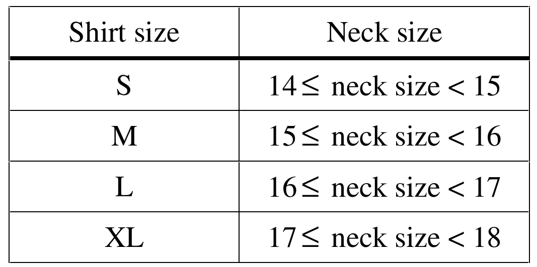
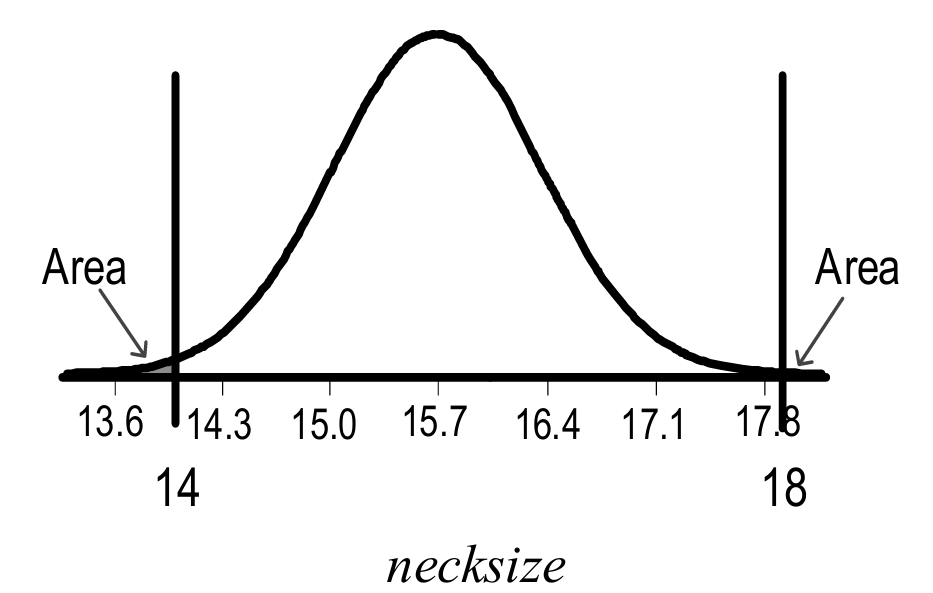
A customer “misses out” if their neck size falls outside the range covered by S through XL, that is, below \(14\) inches or at \(18\) inches or above. So we need two tail probabilities:
\( P(\text{neck size}<14 \text{ or } \text{neck size}\ge18)=P(\text{neck size}<14)+P(\text{neck size}\ge18) \)
Convert each cutoff to a \(z\)-score using \(z=\dfrac{x-\mu}{\sigma}\):
\( z_1=\dfrac{14-15.7}{0.7}\approx-2.43 \)
\( z_2=\dfrac{18-15.7}{0.7}\approx3.29 \)
From the standard normal table:
\( P(z<-2.43)\approx0.0076 \)
\( P(z>3.29)\approx0.0005 \)
Adding these two tail areas together:
\( 0.0076+0.0005\approx0.0081 \)
\( \boxed{\text{About } 0.81\% \text{ of customers will not find their size.}} \)
(b)
Size M corresponds to neck sizes from \(15\) up to (but not including) \(16\) inches, so we need the area under the normal curve between these two values.
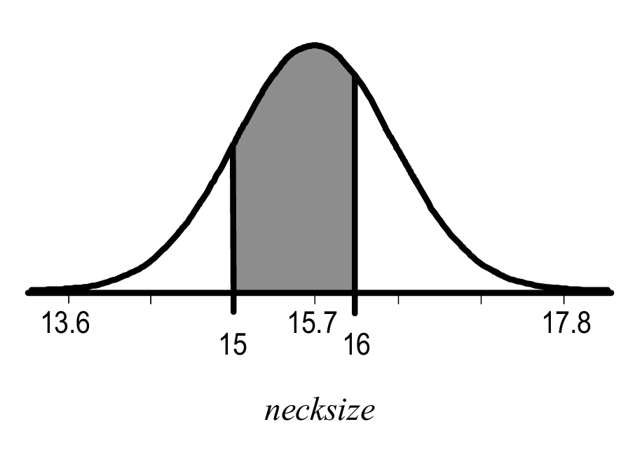
Convert both boundaries to \(z\)-scores:
\( z_1=\dfrac{15-15.7}{0.7}=-1.00 \)
\( z_2=\dfrac{16-15.7}{0.7}\approx0.43 \)
The proportion is the area between these two \(z\)-values:
\( P(-1.00<z<0.43)=P(z<0.43)-P(z<-1.00) \)
\( P(-1.00<z<0.43)\approx0.6664-0.1587 \)
\( P(-1.00<z<0.43)\approx0.5077 \)
\( \boxed{\text{About } 50.77\% \text{ of men wear size M.}} \)
(c)
Each of the \(12\) customers independently either requests size M or doesn’t, with the same probability of “success” each time — that’s a binomial setting. Let \(X\) be the number of customers (out of \(12\)) who request size M.
\( X\sim\text{Binomial}(n=12,\ p=0.5077) \)
We want the probability of exactly \(4\) successes, so we use the binomial formula:
\( P(X=4)=\binom{12}{4}(0.5077)^4(0.4923)^8 \)
Work out each piece separately. The number of ways to choose which \(4\) of the \(12\) customers want size M:
\( \binom{12}{4}=495 \)
The probability that \(4\) specific customers all want M:
\( (0.5077)^4\approx0.0664 \)
The probability that the remaining \(8\) customers all want something else:
\( (0.4923)^8\approx0.00347 \)
Multiply everything together:
\( P(X=4)\approx495\times0.0664\times0.00347 \)
\( P(X=4)\approx0.1139 \)
\( \boxed{P(X=4)\approx0.1139} \)