
AP Statistics 2.12 Sampling Distributions and the Central Limit Theorem- Exam Style Questions - FRQs - New Syllabus
Question
(ii) Suppose Cleo took a random sample of $n=2$ necklaces that resulted in a sample mean amount of gold applied of 303 mg. Would that result indicate that the population mean amount of gold being applied by the machine is different from 300 mg? Justify your answer without performing an inference procedure.
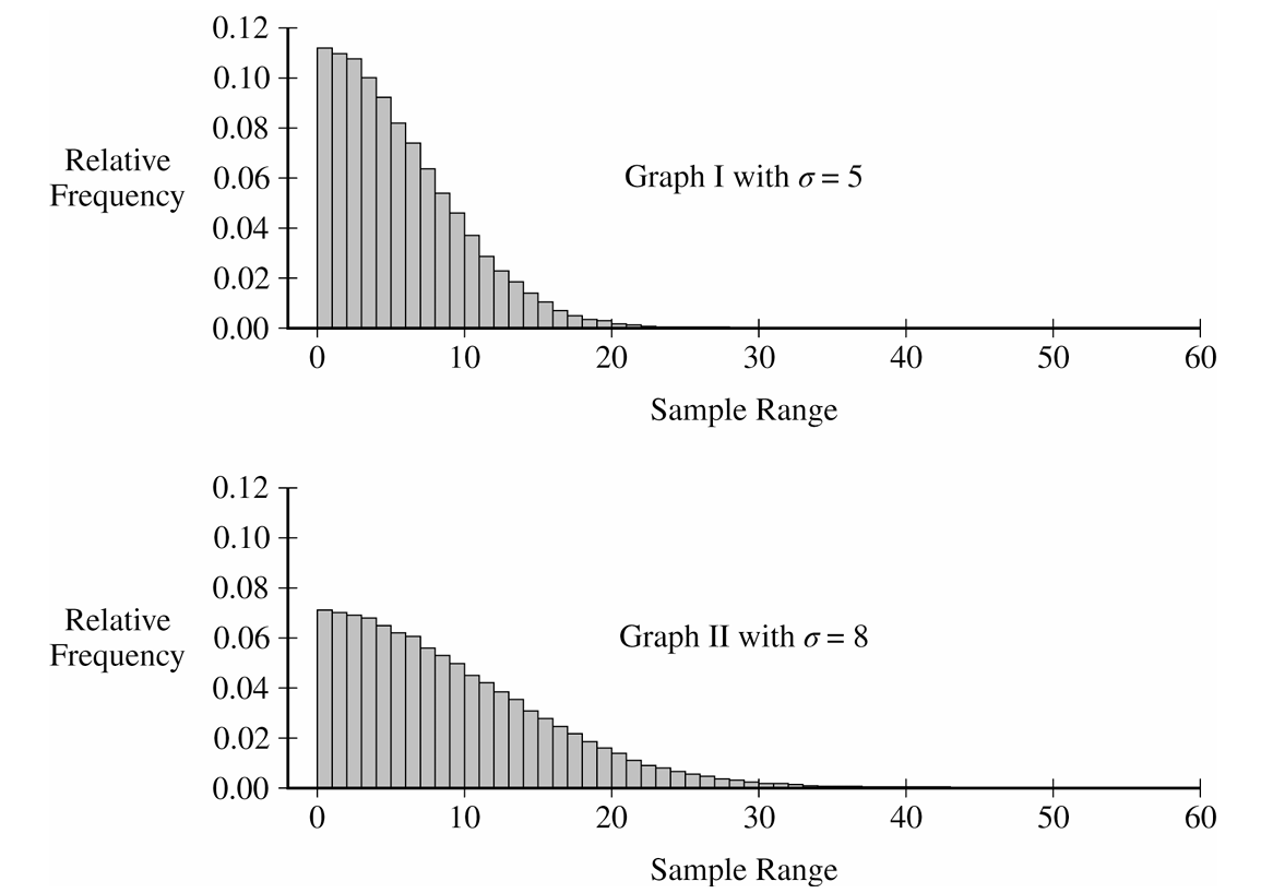
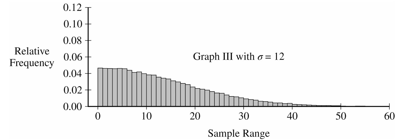
(ii) Describe how the sampling distribution of the sample range for samples of size $n=2$ changes as the value of the population standard deviation increases.
(ii) Do Cleo’s sample mean of 303 mg and range of 10 mg indicate that the machine is not working properly? Explain your answer.
Most-appropriate topic codes (AP Statistics):
• Topic \(2.11\) — The Normal Distribution (Part \( \mathrm{a} \))
• Topic \(2.12\) — Central Limit Theorem and Sampling Distributions for Sample Means (Parts \( \mathrm{b} \), \( \mathrm{d} \))
▶️ Answer/Explanation
(a)
To find the probability, standardize the given values to z-scores using the formula $z = \frac{x – \mu}{\sigma}$.
$P(296 < X < 304) = P\left(\frac{296-300}{5} < Z < \frac{304-300}{5}\right)$
This simplifies to $P(-0.8 < Z < 0.8) \approx 0.5762$.
(b) (i)
For $n=2$, the standard error of the mean is $\sigma_{\bar{x}} = \frac{5}{\sqrt{2}} \approx 3.535$.
$P(\bar{X} > 303) = P\left(Z > \frac{303-300}{3.535}\right) = P(Z > 0.849)$
$P(\bar{X} > 303) \approx 0.198$.
(b) (ii)
No, this result would not indicate the machine is malfunctioning. Because a sample mean of $303$ mg or higher has a probability of approximately $0.198$ (about $20\%$) assuming the machine is working properly, this result is fairly common and not unusual.
(c) (i)
The sampling distribution of the sample range is heavily right-skewed. The center is around a sample range of $4$ to $5$ mg, and the values vary from $0$ mg up to approximately $25$ mg.
(c) (ii)
As the population standard deviation increases, the center of the sampling distribution shifts to the right (indicating a larger expected range), and the distribution becomes more spread out, showing greater variability in the possible sample ranges.
(d) (i)
No, a sample range of $10$ mg is not unusual. Looking at Graph I (where $\sigma=5$), the bars at and to the right of $10$ mg make up a substantial portion of the total area (well over $5\%$), meaning a range of $10$ mg or more occurs quite frequently by chance.
(d) (ii)
No, these results do not indicate a problem. Based on part (b), a sample mean of $303$ mg is not unusual (happens about $20\%$ of the time), and based on part (d)(i), a sample range of $10$ mg is also quite typical. Since neither metric is statistically surprising, there is no convincing evidence to doubt the machine is working properly.
Question
• Calculate and record the median of the sample.
• Repeat the process to obtain a total of \(15,000\) medians.
Most-appropriate topic codes (AP Statistics):
• Topic \(1.12\) — Potential Problems with Sampling (Part \( \mathrm{a} \))
• Topic \(1.7\) — Summary Statistics for One Quantitative Variable (Parts \( \mathrm{b} \), \( \mathrm{d} \), \( \mathrm{e} \))
• Topic \(2.12\) — Central Limit Theorem and Sampling Distributions for Sample Means (Parts \( \mathrm{c} \), \( \mathrm{f} \))
▶️ Answer/Explanation
(a)
Because a random sample was used, it is appropriate to generalize the results to the population of all rental prices for one-bedroom apartments in the city that are listed on this particular website at the time the sample was taken.
(b)
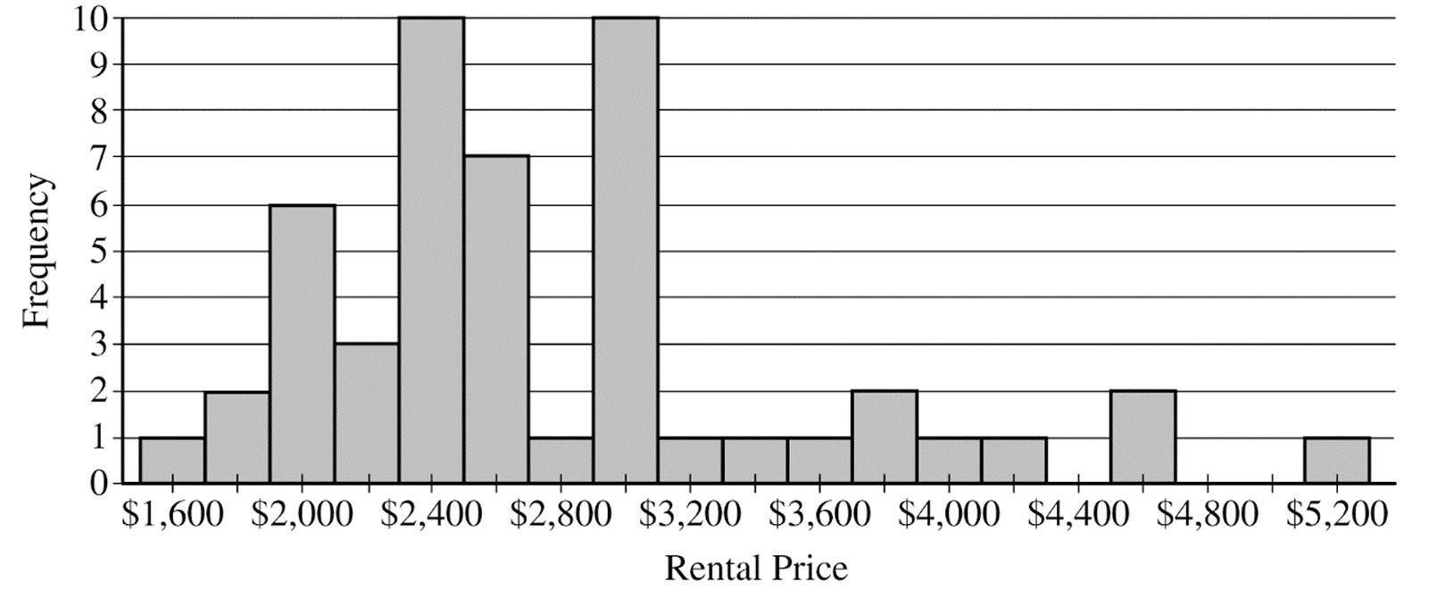
The histogram indicates that the distribution of rental prices is strongly skewed to the right.
Because of this right skewness, the sample mean will be pulled substantially higher by a few very large rental prices.
Consequently, the sample mean would overestimate the typical rental price, whereas the sample median provides a more accurate representation of the center.
(c)
To develop a theoretical sampling distribution, Emma would need to obtain every possible sample of size \(50\) from the population of apartments listed on the website.
She would then compute the median rental price for each of these possible samples.
The entire collection of all these computed sample medians forms the theoretical sampling distribution for the sample median.
(d)
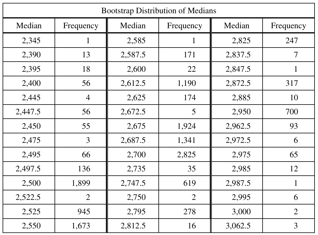
i. The \(5\text{th}\) percentile corresponds to the \((0.05)(15,000) = 750\text{th}\) value in the ordered data.
By keeping a running cumulative total of the frequencies down the columns, the \(750\text{th}\) value first falls in the row for the median of \(\$2,500\).
ii. The \(95\text{th}\) percentile corresponds to the \((0.95)(15,000) = 14,250\text{th}\) value in the ordered data.
Continuing to add the frequencies, the \(14,250\text{th}\) value falls in the row for the median of \(\$2,950\).
(e)
We need to sum the frequencies of all bootstrap medians from \(\$2,500\) to \(\$2,950\) inclusive.
\(\text{Sum} = 1,899 + 2 + \dots + 10 + 700 = 14,404\)
\(\text{Percentage} = \left(\dfrac{14,404}{15,000}\right) \times 100\% \approx 96.03\%\)
(f)
Based on our previous parts, an approximate \(96\%\) confidence interval for the median is \((\$2,500, \$2,950)\).
Interpretation: We are approximately \(96\%\) confident that the true median rental price of all one-bedroom apartments listed on this website for this city is between \(\$2,500\) and \(\$2,950\).
Question
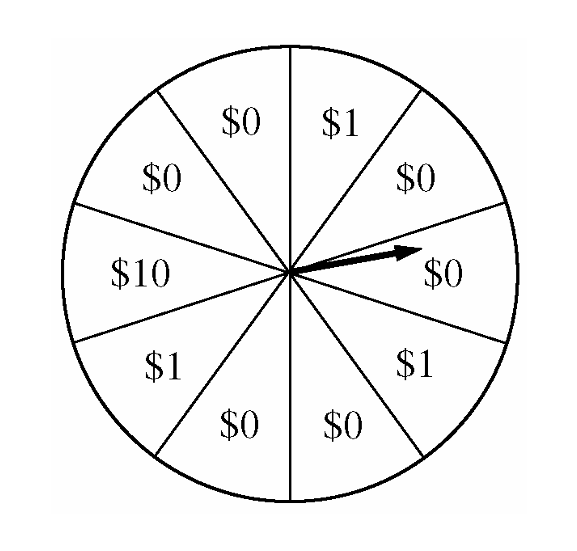

Most-appropriate topic codes (AP Statistics):
• Topic 2.9 — Parameters of Random Variables (Parts b, c)
• Topic 2.12 — Sampling Distributions and the Central Limit Theorem (Part d)
▶️ Answer/Explanation
(a)
The random variable \(X\) is defined as the net contribution to the charity, which is equal to: \(\text{Donation Received} – \text{Payout Amount}\).
• For a payout of \$0, the net contribution is: \(\$2 – \$0 = \$2\). There are 6 sectors labeled \$0 out of 10 total sectors.
• For a payout of \$1, the net contribution is: \(\$2 – \$1 = \$1\). There are 3 sectors labeled \$1 out of 10 total sectors.
• For a payout of \$10, the net contribution is: \(\$2 – \$10 = -\$8\). There is 1 sector labeled \$10 out of 10 total sectors.
The completed probability distribution table is:

(b)
The expected value of the net contribution for a single play is calculated using the formula: \(E(X) = \sum x_i P(x_i)\).
\(E(X) = (\$2)(0.6) + (\$1)(0.3) + (-\$8)(0.1)\)
\(E(X) = 1.2 + 0.3 – 0.8\)
\(E(X) = \$0.70\)
The expected net contribution to the charity per play is \(\$0.70\).
(c)
Let \(n\) be the number of times the game is played.
The total expected net contribution for \(n\) plays is: \(E(\text{Total}) = n \cdot E(X) = 0.70n\).
We want the total expected net contribution to be at least \$500:
\(0.70n \ge 500\)
\(n \ge \dfrac{500}{0.70}\)
\(n \ge 714.29\)
Since the number of plays must be an integer, the game must be played a minimum of \(715\) times.
(d)
Let \(W\) represent the total net contribution from 1,000 plays of the game.
We are given that \(W\) is approximately normally distributed with a mean of \(\mu_W = \$700\) and a standard deviation of \(\sigma_W = \$92.79\).
We want to find the probability that the net contribution is at least \$500: \(P(W \ge 500)\).
First, compute the standardized \(z\)-score:
\(z = \dfrac{500 – \mu_W}{\sigma_W} = \dfrac{500 – 700}{92.79} = \dfrac{-200}{92.79} \approx -2.16\)
Using the standard normal probability table, the probability lying below \(z = -2.16\) is \(0.0154\).
Therefore, the probability of obtaining a net contribution of at least \$500 is:
\(P(Z \ge -2.16) = 1 – 0.0154 = 0.9846\).
The normal approximation for the probability is approximately \(0.9846\).
Question
Most-appropriate topic codes (AP Statistics):
• Topic 2.12 — Sampling Distributions and the Central Limit Theorem (Part a)
• Topic 4.1 — Sampling Distributions for Sample Means (Part b)
▶️ Answer/Explanation
(a)
The sampling distribution of the sample mean song length $\overline{X}$ can be described completely by three attributes:
Center: The mean of the sampling distribution is equal to the population mean, so $\mu_{\overline{X}} = \mu = 3.9\text{ minutes}$.
Spread: The standard deviation of the sampling distribution is computed using the population standard deviation divided by the square root of the sample size:
$\sigma_{\overline{X}} = \dfrac{\sigma}{\sqrt{n}} = \dfrac{1.1}{\sqrt{40}} \approx 0.174\text{ minutes}$
Shape: Since the sample size $n = 40$ is sufficiently large ($n \ge 30$), the Central Limit Theorem applies directly. Even though the original population distribution is non-normal, the shape of the sampling distribution of the sample mean will be approximately normal.
(b)
The probability that the total airtime of 40 randomly selected songs exceeds the available time (that is, the probability that the total airtime of 40 randomly selected songs is greater than 160 minutes) is equivalent to the probability that the sample mean length of the 40 songs is greater than $\dfrac{160}{40} = 4.0$ minutes.
According to part (a), the distribution of the sample mean length $\overline{X}$ is approximately normal. Therefore,
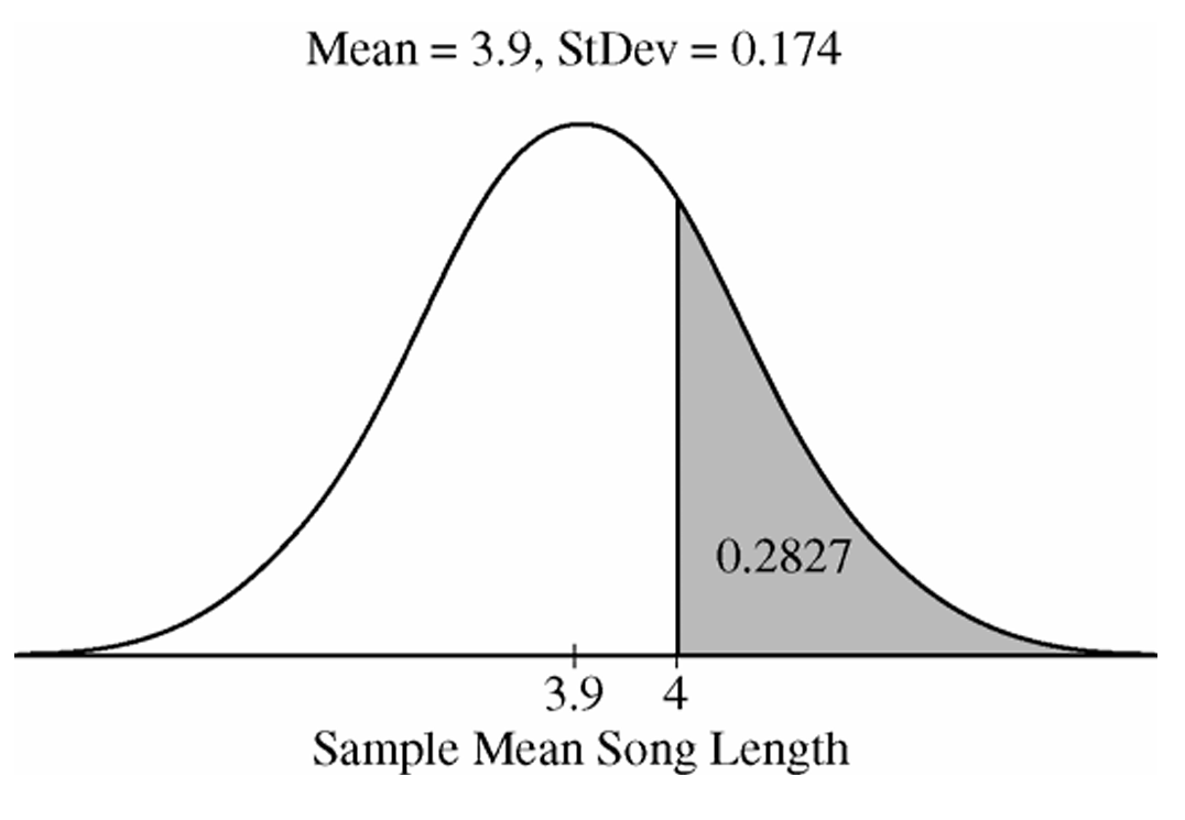
$P(\overline{X} > 4.0) \approx P\left( Z > \dfrac{4.0 – 3.9}{0.174} \right) = P(Z > 0.57) = 1 – 0.7157 = 0.2843$.
(The calculator gives the answer as 0.2827.)
The approximate sampling distribution of the sample mean song length and the desired probability are displayed below.
Question
Most-appropriate topic codes (AP Statistics):
• Topic \(2.10\) — The Binomial Distribution (Part \(\mathrm{b}\))
• Topic \(2.12\) — Sampling Distributions and the Central Limit Theorem (Part \(\mathrm{c}\))
▶️ Answer/Explanation
(a)
Let \(X\) denote the stopping distance. We are told that \(X\) is normally distributed with
\( \mu_X = 125 \text{ ft}, \qquad \sigma_X = 6.5 \text{ ft} \)
We want the value \(x\) such that \(P(X \leq x) = 0.70\).
From the standard normal table, the \(z\)-score with a cumulative probability of \(0.70\) is
\( z = 0.52 \)
Using the \(z\)-score formula and solving for \(x\):
\( z = \dfrac{x – \mu}{\sigma} \implies x = \mu + z\sigma \)
\( x = 125 + 0.52(6.5) = 125 + 3.38 \)
\( \boxed{x \approx 128.4 \text{ feet}} \)
So the 70th percentile of the stopping distance distribution is approximately \(128.4\) feet — meaning \(70\%\) of cars stop within this distance.
(b)
From part (a), a stopping distance greater than \(128.4\) feet corresponds to the top \(30\%\) of the distribution:
\( p = P(X > 128.4) = 1 – 0.70 = 0.30 \)
Let \(Y\) = number of cars (out of 5) that stop in a distance greater than \(128.4\) feet. Since each car is independent and the probability of “success” is the same for each, \(Y\) follows a binomial distribution:
\( Y \sim B(n=5,\ p=0.30) \)
We need \(P(Y \geq 2)\). It is easier to use the complement:
\( P(Y \geq 2) = 1 – P(Y \leq 1) = 1 – \bigl[P(Y=0) + P(Y=1)\bigr] \)
\( P(Y=0) = \binom{5}{0}(0.30)^0(0.70)^5 = 1 \cdot 1 \cdot 0.16807 = 0.16807 \)
\( P(Y=1) = \binom{5}{1}(0.30)^1(0.70)^4 = 5 \cdot 0.30 \cdot 0.2401 = 0.36015 \)
\( P(Y \leq 1) = 0.16807 + 0.36015 = 0.52822 \)
\( P(Y \geq 2) = 1 – 0.52822 \)
\( \boxed{P(Y \geq 2) \approx 0.4718} \)
There is roughly a \(47.18\%\) chance that at least 2 of the 5 randomly selected cars will stop beyond \(128.4\) feet — think of it as just under a coin-flip, which makes intuitive sense since each car has a \(30\%\) chance on its own.
(c)
Let \(\bar{X}\) denote the mean stopping distance of a random sample of \(n = 5\) cars. Because the individual stopping distances are normally distributed, the sampling distribution of \(\bar{X}\) is also exactly normal with:
\( \mu_{\bar{X}} = \mu = 125 \text{ ft} \)
\( \sigma_{\bar{X}} = \dfrac{\sigma}{\sqrt{n}} = \dfrac{6.5}{\sqrt{5}} \approx 2.907 \text{ ft} \)
We want \(P(\bar{X} \geq 130)\). Convert to a \(z\)-score:
\( z = \dfrac{130 – 125}{6.5/\sqrt{5}} = \dfrac{5}{2.907} \approx 1.72 \)
\( P(\bar{X} \geq 130) = P(Z \geq 1.72) = 1 – P(Z < 1.72) \)
\( P(Z < 1.72) \approx 0.9573 \)
\( P(\bar{X} \geq 130) = 1 – 0.9573 \)
\( \boxed{P(\bar{X} \geq 130) \approx 0.0427} \)
There is only about a \(4.27\%\) chance that the average stopping distance for 5 randomly selected cars exceeds 130 feet — this is much smaller than the \(30\%\) chance for any single car, because averaging over 5 cars reduces variability considerably and makes extreme means much less likely.
Question
How can you tell?
Explain your choice.
Explain your choice.
Most-appropriate topic codes (AP Statistics):
• Topic 2.12 — Sampling Distributions and the Central Limit Theorem (Part \(\mathrm{a}\))
▶️ Answer/Explanation
(a)
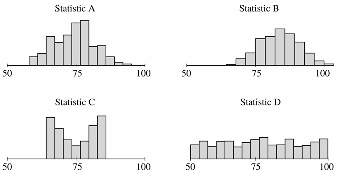
Statistics \(A\), \(C\), and \(D\) appear to be unbiased estimators of the population parameter.
An estimator is said to be unbiased if the mean (center) of its sampling distribution equals the true population parameter. In other words, there is no systematic tendency to overestimate or underestimate.
For Statistics \(A\), \(C\), and \(D\), the distributions appear to be centered at approximately \(\mu_{\text{stat}} \approx 75\), which equals the true population parameter value of \(75\).
For Statistic \(B\), the distribution is centered at approximately \(85\), which is clearly greater than \(75\), so Statistic \(B\) is a biased estimator — it consistently overestimates the parameter.
\(\boxed{\text{Unbiased estimators: Statistics } A,\ C,\ \text{and } D}\)
(b)
Statistic \(A\) would be the better estimator between \(A\) and \(B\).
Statistic \(B\) is centered at approximately \(85\), which is far from the true parameter value of \(75\) — it is a biased estimator that systematically overestimates.
Statistic \(A\), on the other hand, is centered at approximately \(75\), making it an unbiased estimator. Both \(A\) and \(B\) have roughly similar variability (spread), but since only \(A\) is centered at the true parameter, \(A\) will consistently produce estimates closer to \(75\).
\(\boxed{\text{Statistic } A \text{ is the better estimator}}\)
(c)
Statistic \(C\) would be the better estimator between \(C\) and \(D\).
Both Statistics \(C\) and \(D\) appear to be unbiased — their distributions are each centered at approximately \(75\), the true population parameter value. So bias is not a distinguishing factor here.
However, the two differ substantially in variability. Statistic \(C\) has a much smaller spread (lower variance), meaning its estimates cluster tightly around \(75\). Statistic \(D\) has a very large spread, so its individual estimates can deviate far from \(75\), even though on average they are correct.
Since both estimators are unbiased, the one with lower variability is preferred — it will produce more precise estimates in practice.
\(\boxed{\text{Statistic } C \text{ is the better estimator}}\)
Question
Most-appropriate topic codes (AP Statistics):
• Topic 4.1 — Sampling Distributions for Sample Means (Part \(\mathrm{a}\))
• Topic 2.11 — The Normal Distribution (Part \(\mathrm{b}\))
▶️ Answer/Explanation
(a)
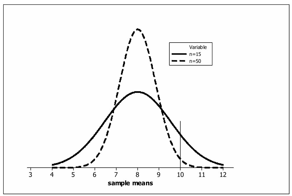
A random sample of \(n = 15\) fish is more likely to have a sample mean greater than 10 inches.
Both sampling distributions are centered at the true mean \(\mu = 8\) inches, but they differ in their variability. The standard deviation of the sampling distribution of the sample mean is given by \(\dfrac{\sigma}{\sqrt{n}}\), so a smaller sample size produces a larger standard deviation — meaning the distribution is more spread out.
Since the sampling distribution for \(n = 15\) is more spread out than for \(n = 50\), the tail area beyond 10 inches is larger for \(n = 15\), making it more likely to observe a sample mean greater than 10 inches with the smaller sample.
\(\boxed{P(\bar{x} > 10 \mid n=15) > P(\bar{x} > 10 \mid n=50) \text{ because the } n=15 \text{ distribution has greater variability.}}\)
(b)
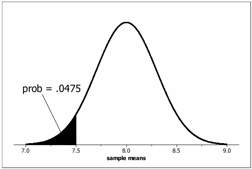
We are given: \(\mu = 8\), \(\sigma_{\bar{x}} = 0.3\), and we want \(P(\bar{x} < 7.5)\).
First, compute the \(z\)-score:
\(z = \dfrac{\bar{x} – \mu}{\sigma_{\bar{x}}} = \dfrac{7.5 – 8}{0.3} = \dfrac{-0.5}{0.3} \approx -1.67\)
Now look up the standard normal table for \(z = -1.67\):
\(P(\bar{x} < 7.5) = P(z < -1.67) \approx 0.0475\)
\(\boxed{P(\bar{x} < 7.5) \approx 0.0475}\)
(c)
Yes, it would still be appropriate to use the normal distribution to compute this probability.
By the Central Limit Theorem (CLT), the sampling distribution of the sample mean \(\bar{x}\) is approximately normal for sufficiently large sample sizes, regardless of the shape of the population distribution.
Since our sample size is \(n = 50\), which is reasonably large (generally \(n \geq 30\) is considered sufficient), the CLT guarantees that \(\bar{x}\) follows an approximately normal distribution even if the individual fish lengths are nonnormally distributed.
Therefore, the probability calculated in part (b) remains a good approximation.
\(\boxed{\text{Yes — by the CLT, } n = 50 \text{ is large enough for the sampling distribution of } \bar{x} \text{ to be approximately normal.}}\)
Question
Most-appropriate topic codes (AP Statistics):
• Topic 2.10 — The Binomial Distribution (Part \(\mathrm{b}\))
• Topic 2.8 — Introduction to Random Variables and Probability Distributions (Parts \(\mathrm{a}\), \(\mathrm{b}\))
• Topic 2.12 — Sampling Distributions and the Central Limit Theorem (Part \(\mathrm{c}\))
• Topic 4.1 — Sampling Distributions for Sample Means (Part \(\mathrm{c}\))
▶️ Answer/Explanation
(a)
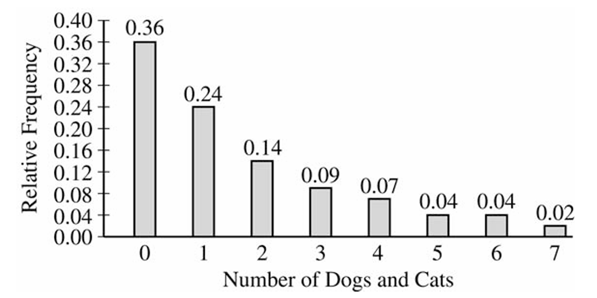
A household is in violation if it owns more than \(3\) pets, i.e., \(X > 3\). Read the relative frequencies for \(X = 4, 5, 6, 7\) directly from the graph and add them up.
\(P(X > 3) = P(X=4) + P(X=5) + P(X=6) + P(X=7)\)
\(P(X > 3) = 0.07 + 0.04 + 0.04 + 0.02\)
\(\boxed{P(X > 3) = 0.17}\)
(b)
Let \(Y\) = the number of households in violation among the \(10\) selected. Since each household is independently either in violation or not, \(Y\) follows a binomial distribution with \(n = 10\) and \(p = 0.17\) (from part (a)).
Using the binomial probability formula \(P(Y = k) = \dbinom{n}{k} p^k (1-p)^{n-k}\):
\(P(Y = 2) = \binom{10}{2}(0.17)^2(0.83)^8\)
\(P(Y = 2) = 45 \times (0.0289) \times (0.2252)\)
\(\boxed{P(Y = 2) \approx 0.2929}\)
(c)
Because the sample size \(n = 150\) is large, the Central Limit Theorem tells us the sampling distribution of \(\bar{X}\) will be approximately normal, regardless of the shape of the original population distribution.
The mean of the sampling distribution equals the population mean:
\(\mu_{\bar{X}} = \mu = 1.65\)
The standard deviation (standard error) of the sampling distribution is:
\(\sigma_{\bar{X}} = \dfrac{\sigma}{\sqrt{n}} = \dfrac{1.851}{\sqrt{150}} \approx 0.1511\)
So the sampling distribution of \(\bar{X}\) is approximately \(N(1.65,\ 0.1511)\) — normal, centered at \(1.65\), with a standard deviation of about \(0.1511\).
Question
Most-appropriate topic codes (AP Statistics):
• Topic 2.7 — Independent Events and Unions of Events (Part \(\mathrm{b}\))
• Topic 2.12 — Sampling Distributions and the Central Limit Theorem (Part \(\mathrm{c}\))
▶️ Answer/Explanation
(a)
Since \(M = D + E\) is a normal random variable plus a constant, \(M\) is also normally distributed.
With true depth \(D = 2\) feet, the distribution of \(M\) has:
\(\mu_M = 2\,\text{feet}, \qquad \sigma_M = 1.5\,\text{feet}\)
We want \(P(M < 0)\). Standardizing:
\(P(M < 0) = P\!\left(Z < \frac{0 – 2}{1.5}\right) = P(Z < -1.33)\)
Using the standard normal table:
\(\boxed{P(M < 0) \approx 0.0918}\)
(b)
Let each individual measurement be negative with probability \(p = 0.0918\) (from part (a)), and let the three measurements be independent.
Using the complement rule — it is easier to find the probability that none of the three measurements is negative, then subtract from 1:
\(P(\text{at least one negative}) = 1 – P(\text{none negative})\)
\(= 1 – (1 – 0.0918)^3\)
\(= 1 – (0.9082)^3\)
\(= 1 – 0.7491\)
\(\boxed{P(\text{at least one negative}) \approx 0.2509}\)
(c)
Let \(\bar{X}\) denote the mean of three independent depth measurements where the true depth is \(2\) feet.
Since each measurement is normally distributed, the sampling distribution of \(\bar{X}\) is also normal with:
\(\mu_{\bar{X}} = 2\,\text{feet}, \qquad \sigma_{\bar{X}} = \frac{1.5}{\sqrt{3}} = 0.8660\,\text{feet}\)
We want \(P(\bar{X} < 0)\). Standardizing:
\(P(\bar{X} < 0) = P\!\left(Z < \frac{0 – 2}{1.5/\sqrt{3}}\right) = P\!\left(Z < \frac{-2}{0.8660}\right) = P(Z < -2.31)\)
Using the standard normal table:
\(\boxed{P(\bar{X} < 0) \approx 0.0104}\)
Question

Most-appropriate topic codes (AP Statistics):
• Topic 4.5 — Carrying Out a Test for a Population Mean or Population Mean Difference (Parts \(\mathrm{b}\), \(\mathrm{c}\), \(\mathrm{d}\))
• Topic 2.12 — Sampling Distributions and the Central Limit Theorem (Parts \(\mathrm{e}\), \(\mathrm{f}\))
▶️ Answer/Explanation
(a)
Let \(\sigma^2\) denote the true population variance of the readings of recently manufactured thermostats (in degrees Fahrenheit squared).
\(H_0: \sigma^2 = 1.52 \qquad \text{(variance has not changed)}\)
\(H_a: \sigma^2 > 1.52 \qquad \text{(recently produced thermostats are more variable)}\)
(b)
First, compute the sample standard deviation from the 10 readings:
\(s^2 = 2.0383 \implies s = 1.4277\)
Then compute the test statistic:
\(\chi^2 = \frac{(n-1)s^2}{1.52} = \frac{9 \times 2.0383}{1.52} = \frac{18.345}{1.52}\)
\(\boxed{\chi^2 \approx 12.069}\)
(c)
Under \(H_0\), the test statistic follows a \(\chi^2\) distribution with \(n – 1 = 9\) degrees of freedom.
The \(p\)-value is the probability of obtaining a test statistic as large as or larger than the observed value:
\(p\text{-value} = P\!\left(\chi^2_9 \geq 12.069\right) \approx 0.2094\)
(From the table: \(0.20 < p\text{-value} < 0.25\))
Since the \(p\)-value \(\approx 0.2094 > 0.05\), we fail to reject \(H_0\). There is not statistically significant evidence at the \(\alpha = 0.05\) level that the recently manufactured thermostats have become more variable than in the past.
\(\boxed{\text{Fail to reject } H_0;\ p\text{-value} \approx 0.209}\)
(d)
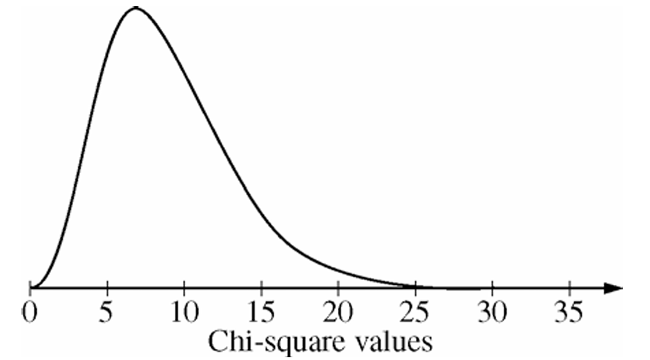
The smallest value of the test statistic that leads to rejection of \(H_0\) at the 5% significance level is the 95th percentile of the \(\chi^2\) distribution with 9 degrees of freedom:
\(\boxed{\chi^2_{0.05,\,9} = 16.92}\)
The rejection region consists of all chi-square values greater than or equal to \(16.92\), which corresponds to the shaded right tail of the \(\chi^2_9\) curve (as marked on the graph above).
(e)
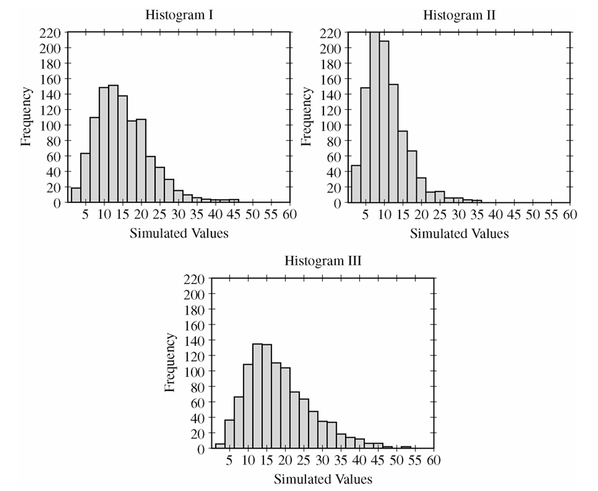
The rejection region — all simulated values to the right of \(16.92\) — should be marked on each of the three histograms (Histogram I, Histogram II, and Histogram III) as indicated by the dashed vertical lines in the diagrams above.
(f)
Largest variance → Histogram III. A population with a larger variance will tend to produce larger sample variances \(s^2\), and hence larger values of the test statistic \(\frac{(n-1)s^2}{1.52}\). Histogram III has the greatest proportion of simulated values falling to the right of \(16.92\) — meaning it has the highest probability of correctly rejecting \(H_0\) — so it corresponds to the population with the largest variance.
Smallest variance → Histogram II. Histogram II has its simulated values concentrated most tightly at smaller values, with the smallest proportion of values exceeding \(16.92\). This means it has the lowest probability of rejecting \(H_0\), consistent with coming from the population whose variance is smallest (and closest to \(1.52\) among the three).
\(\boxed{\text{Largest variance: Histogram III} \qquad \text{Smallest variance: Histogram II}}\)
Question
Most-appropriate topic codes (AP Statistics):
• Topic 4.5 — Carrying Out a Test for a Population Mean or Population Mean Difference (Parts \(\mathrm{b}\), \(\mathrm{c}\), \(\mathrm{d}\))
• Topic 2.12 — Sampling Distributions and the Central Limit Theorem (Parts \(\mathrm{e}\), \(\mathrm{f}\))
▶️ Answer/Explanation
(a)
Let \(\sigma^2\) denote the true population variance of the readings of recently manufactured thermostats (in degrees Fahrenheit squared).
\(H_0: \sigma^2 = 1.52 \qquad \text{(variance has not changed)}\)
\(H_a: \sigma^2 > 1.52 \qquad \text{(recently produced thermostats are more variable)}\)
(b)
First, compute the sample standard deviation from the 10 readings:
\(s^2 = 2.0383 \implies s = 1.4277\)
Then compute the test statistic:
\(\chi^2 = \frac{(n-1)s^2}{1.52} = \frac{9 \times 2.0383}{1.52} = \frac{18.345}{1.52}\)
\(\boxed{\chi^2 \approx 12.069}\)
(c)
Under \(H_0\), the test statistic follows a \(\chi^2\) distribution with \(n – 1 = 9\) degrees of freedom.
The \(p\)-value is the probability of obtaining a test statistic as large as or larger than the observed value:
\(p\text{-value} = P\!\left(\chi^2_9 \geq 12.069\right) \approx 0.2094\)
(From the table: \(0.20 < p\text{-value} < 0.25\))
Since the \(p\)-value \(\approx 0.2094 > 0.05\), we fail to reject \(H_0\). There is not statistically significant evidence at the \(\alpha = 0.05\) level that the recently manufactured thermostats have become more variable than in the past.
\(\boxed{\text{Fail to reject } H_0;\ p\text{-value} \approx 0.209}\)
(d)
The smallest value of the test statistic that leads to rejection of \(H_0\) at the 5% significance level is the 95th percentile of the \(\chi^2\) distribution with 9 degrees of freedom:
\(\boxed{\chi^2_{0.05,\,9} = 16.92}\)
The rejection region consists of all chi-square values greater than or equal to \(16.92\), which corresponds to the shaded right tail of the \(\chi^2_9\) curve (as marked on the graph above).
(e)
The rejection region — all simulated values to the right of \(16.92\) — should be marked on each of the three histograms (Histogram I, Histogram II, and Histogram III) as indicated by the dashed vertical lines in the diagrams above.
(f)
Largest variance → Histogram III. A population with a larger variance will tend to produce larger sample variances \(s^2\), and hence larger values of the test statistic \(\frac{(n-1)s^2}{1.52}\). Histogram III has the greatest proportion of simulated values falling to the right of \(16.92\) — meaning it has the highest probability of correctly rejecting \(H_0\) — so it corresponds to the population with the largest variance.
Smallest variance → Histogram II. Histogram II has its simulated values concentrated most tightly at smaller values, with the smallest proportion of values exceeding \(16.92\). This means it has the lowest probability of rejecting \(H_0\), consistent with coming from the population whose variance is smallest (and closest to \(1.52\) among the three).
\(\boxed{\text{Largest variance: Histogram III} \qquad \text{Smallest variance: Histogram II}}\)
Question

Most-appropriate topic codes (AP Statistics):
• Topic 2.12 — Sampling Distributions and the Central Limit Theorem (Part \(\mathrm{b}\))
• Topic 1.7 — Summary Statistics for One Quantitative Variable (Part \(\mathrm{c}\))
• Topic 1.9 — Comparisons of the Distributions for One Quantitative Variable (Part \(\mathrm{d}\))
▶️ Answer/Explanation
(a)
The expected value of a discrete random variable is found by multiplying each value by its probability and adding the results:
\( E(X)=\sum x_i\,p(x_i) \)
Plugging in the values from the table:
\( E(X)=0(0.35)+1(0.20)+2(0.15)+3(0.15)+4(0.10)+5(0.05) \)
\( E(X)=0+0.20+0.30+0.45+0.40+0.25 \)
\( \boxed{E(X)=1.6} \)
(b)
Both sample averages are estimates of the same population mean, \(\mu_X=1.6\), so they should be centered around the same value. What changes is how precise that estimate is.
The standard deviation of a sample mean is
\( \sigma_{\bar{x}}=\dfrac{\sigma}{\sqrt{n}} \)
Since \(1{,}000>20\), a sample of 1,000 days has a much smaller standard deviation for its average, meaning the sample average will tend to land closer to 1.6 than the first sample’s average of 1.25 did.
\( \boxed{\text{The new average should be closer to } 1.6\text{ than }1.25\text{, since larger samples have less variability}} \)
(c)
To find the median, build up the cumulative probabilities:
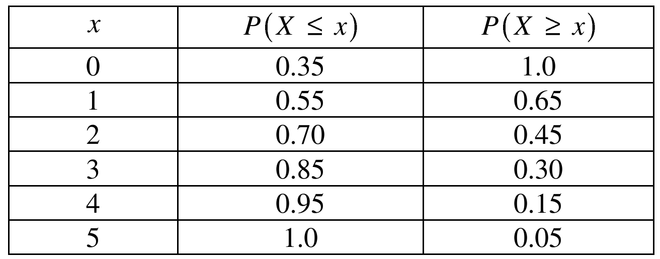
At \(x=1\), both \(P(X\le 1)=0.55\ge 0.5\) and \(P(X\ge 1)=0.65\ge 0.5\) are satisfied. At \(x=2\), \(P(X\ge 2)=0.45<0.5\), so \(x=2\) does not work.
\( \boxed{\text{Median} = 1} \)
(d)
Looking at the table, most of the probability is piled up at the small values (0, 1, 2) with a long tail of smaller probabilities stretching out to 4 and 5. This makes the distribution right-skewed, which pulls the mean up above the median — here the mean of 1.6 is noticeably larger than the median of 1, which is exactly the pattern you’d expect for a distribution skewed toward larger values.
\( \boxed{\text{The distribution is right-skewed, so the mean (1.6) is greater than the median (1)}} \)
Question
Most-appropriate topic codes (AP Statistics):
• Topic 2.12 — Sampling Distributions and the Central Limit Theorem (Parts c, d)
▶️ Answer/Explanation
(a)
Let \(X\) = weight of ore in a randomly selected car. Since \(X \sim N(\mu = 70,\ \sigma = 0.9)\), we standardize:
\(P(X > 70.7) = P\!\left(Z > \frac{70.7 – 70}{0.9}\right) = P(Z > 0.78) = 1 – 0.7823 = \boxed{0.2177}\)
So there is approximately a \(21.77\%\) chance that a single randomly selected car will be loaded with 70.7 tons or more when the equipment is working properly.
(b)
No, a single car weight of 70.7 tons would not give strong reason to suspect overfilling. From part (a), roughly \(22\%\) of all cars — about 1 in every 5 — would weigh 70.7 tons or more even when the equipment is functioning properly. Since this is not an unusually rare event, a single observation of 70.7 tons is not convincing evidence that the loading mechanism is overfilling.
(c)
For a random sample of \(n = 10\) cars, the sampling distribution of the sample mean \(\bar{X}\) has:
\(\mu_{\bar{X}} = 70, \qquad \sigma_{\bar{X}} = \frac{\sigma}{\sqrt{n}} = \frac{0.9}{\sqrt{10}} \approx 0.285\)
Standardizing:
\(P(\bar{X} > 70.7) = P\!\left(Z > \frac{70.7 – 70}{\dfrac{0.9}{\sqrt{10}}}\right) = P\!\left(Z > \frac{0.7}{0.285}\right) = P(Z > 2.46) = 1 – 0.9931 = \boxed{0.0069}\)
So there is only about a \(0.69\%\) chance of observing a sample mean of 70.7 tons or more in a sample of 10 cars when the equipment is functioning properly.
(d)
Yes, a sample mean of 70.7 tons from 10 cars would give good reason to suspect overfilling. From part (c), the probability of this outcome occurring by chance alone — when the equipment is working properly — is only about \(0.0069\), or less than 1 in 100. Such a small probability makes the observed result very unlikely under normal operating conditions, so it is reasonable to suspect the loading mechanism is overfilling the cars.