AP Statistics 2.2 Summary Statistics for Two Categorical Variables- Exam Style Questions - FRQs - New Syllabus

Question

Baseball cards are trading cards that feature data on a player’s performance in baseball games. Michelle is at a national baseball card collector’s convention with approximately $20,000$ attendees. She notices that some collectors have both regular cards, which are easily obtained, and rare cards, which are harder to obtain. Michelle believes that there is a relationship between the number of months a collector has been collecting baseball cards and whether the majority of the cards (cards appearing more often) in their collection are regular or rare. She obtains information from a random sample of $500$ baseball card collectors at the convention and records how many full months they have been collecting baseball cards and whether the majority of the cards in their card collection are regular or rare. Her results are displayed in a two-way table.

Majority Type of Baseball Cards and Months of Collecting Baseball Cards

(a) If one collector from the sample is selected at random, what is the probability that the collector has been collecting baseball cards for $11$ or more months and has a majority of regular baseball cards? Show your work.

(b) Given that a randomly selected collector from the sample has been collecting baseball cards for fewer than $6$ months, what is the probability the collector has a majority of regular baseball cards? Show your work.

(c) Michelle believes there is a relationship between the number of months spent collecting baseball cards and which type of card is the majority in the collection (regular or rare).

i. Name the hypothesis test Michelle should use to investigate her belief. Do not perform the hypothesis test.
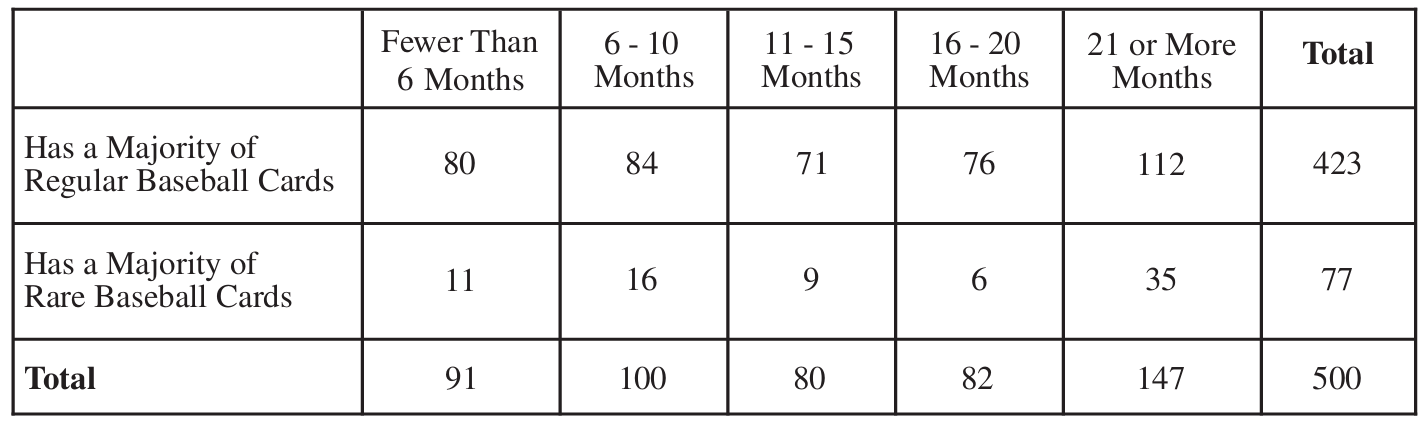
ii. State the appropriate null and alternative hypotheses for the hypothesis test you identified in (c-i). Do not perform the hypothesis test.

(d) After completing the hypothesis test described in part (c), Michelle obtains a $p$-value of $0.0075$. Assuming the conditions for inference are met, what conclusion should Michelle make about her belief? Justify your response.

Most-appropriate topic codes (AP Statistics):

• Topic $2.2$ — Summary Statistics for Two Categorical Variables (Parts $ \mathrm{a} $, $ \mathrm{b} $)
• Topic $3.14$ — Setting Up a Chi-Square Test for Homogeneity or Independence (Part $ \mathrm{c} $)
• Topic $3.15$ — Carrying Out a Chi-Square Test for Homogeneity or Independence (Part $ \mathrm{d} $)

▶️ Answer/Explanation

(a)
To find this probability, we sum the number of collectors who have a majority of regular cards AND have been collecting for $11$ or more months (which covers the $11-15$, $16-20$, and $21+$ columns).
Number of collectors $= 71 + 76 + 112 = 259$.
$P(\ge 11\text{ months and majority regular}) = \dfrac{259}{500} = 0.518$.

(b)
This is a conditional probability. We restrict our focus entirely to the column representing collectors with fewer than $6$ months of collecting, which gives us a new total of $91$ collectors.
Out of those $91$ collectors, $80$ have a majority of regular baseball cards.
$P(\text{majority regular} \mid < 6\text{ months}) = \dfrac{80}{91} \approx 0.879$.

(c)
i. Because Michelle took a single random sample and is comparing two categorical variables from that single sample, she should use a chi-square test for independence.
ii. Null Hypothesis ($H_0$): There is no association between the number of months spent collecting baseball cards and majority card status for all baseball card collectors at the convention.
Alternative Hypothesis ($H_a$): There is an association between the number of months spent collecting baseball cards and majority card status for all baseball card collectors at the convention.

(d)
Because the $p$-value of $0.0075$ is smaller than any reasonable significance level (such as $\alpha = 0.05$), Michelle should reject the null hypothesis.
The data provide convincing statistical evidence that there is a relationship between the number of months spent collecting baseball cards and which type of card is the majority in the collection for all baseball card collectors at the convention.

Question

A local elementary school decided to sell bottles printed with the school district’s logo as a fund-raiser. The students in the elementary school were asked to sell bottles in three different sizes (small, medium, and large). The relative frequencies of the number of bottles sold for each size by the elementary school were $0.5$ for small bottles, $0.3$ for medium bottles, and $0.2$ for large bottles.

A local middle school also decided to sell bottles as a fund-raiser, using the same three sizes (small, medium, and large). The middle school students sold three times the number of bottles that the elementary school students sold. For the middle school students, the proportion of bottles sold was equal for all three sizes.

(a) Complete the segmented bar graphs representing the relative frequencies of the number of bottles sold for each size by students at each school.

(b) An administrator at the elementary school concluded that the elementary school students sold more small bottles than the middle school students did. Is the elementary school administrator’s conclusion correct? Explain your response.

Two high schools are also selling the bottles and are competing to see which one sold more large bottles.

(c) A mosaic plot for the distribution of the number of bottles sold by each of the high schools is shown here.

i. Which of the two high schools sold a greater proportion of large bottles? Justify your answer.
ii. Which of the two high schools sold a greater number of large bottles? Justify your answer.

Most-appropriate topic codes (AP Statistics):

• Topic $2.1$ — Tabular and Graphical Representations for the Distributions of Two Categorical Variables (Parts $ \mathrm{a} $, $ \mathrm{c} $)
• Topic $2.2$ — Summary Statistics for Two Categorical Variables (Part $ \mathrm{b} $)

▶️ Answer/Explanation

(a)

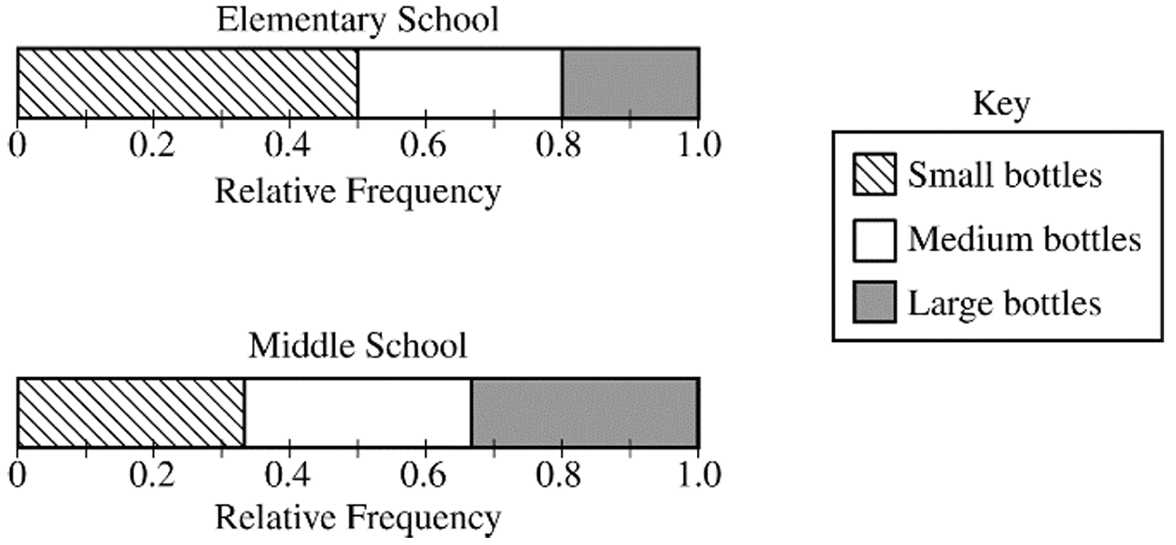
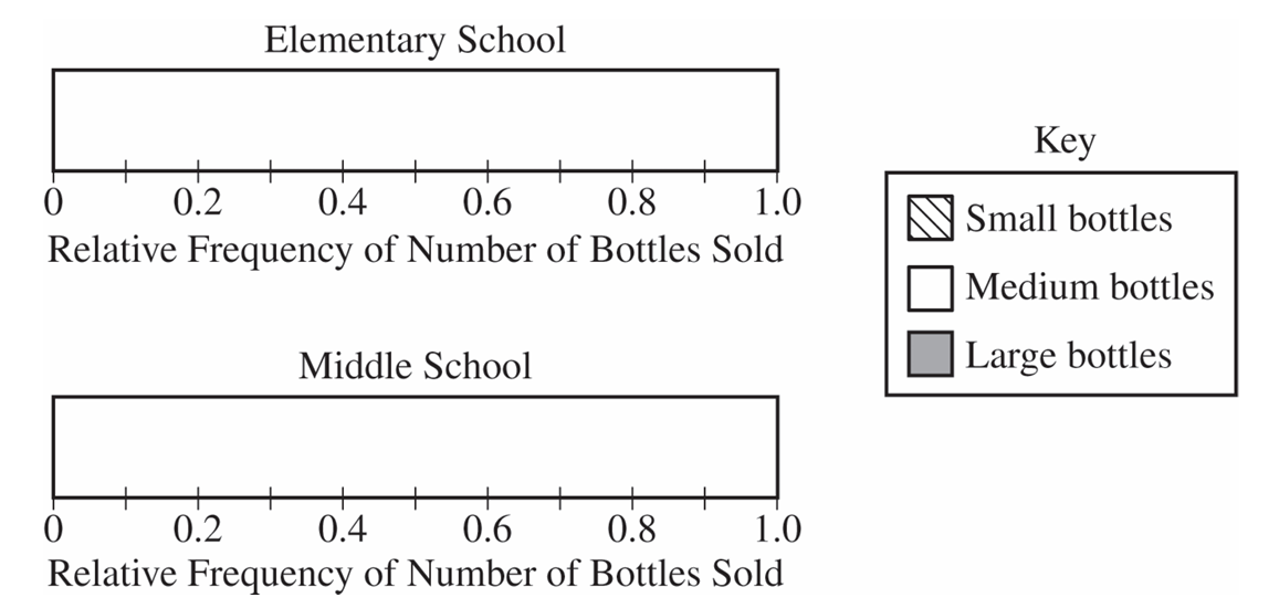
For the Elementary School bar graph, partition the segments at $0.5$ for small bottles, $0.8$ ($0.5 + 0.3$) for medium bottles, and $1.0$ for large bottles.
For the Middle School bar graph, since the proportions are equal, partition the bar into three equal areas at approximately $0.33$ and $0.67$.

(b)
No, the elementary school administrator’s conclusion is incorrect.
Let $x$ represent the total number of bottles sold by the elementary school.
This means the elementary school sold $0.5x$ small bottles.
The middle school sold three times as many total bottles, which is $3x$.
Since the proportion is equal across the three sizes, the middle school sold $\frac{1}{3}(3x) = x$ small bottles.
Because $x > 0.5x$, the middle school actually sold more small bottles than the elementary school.

(c)(i)
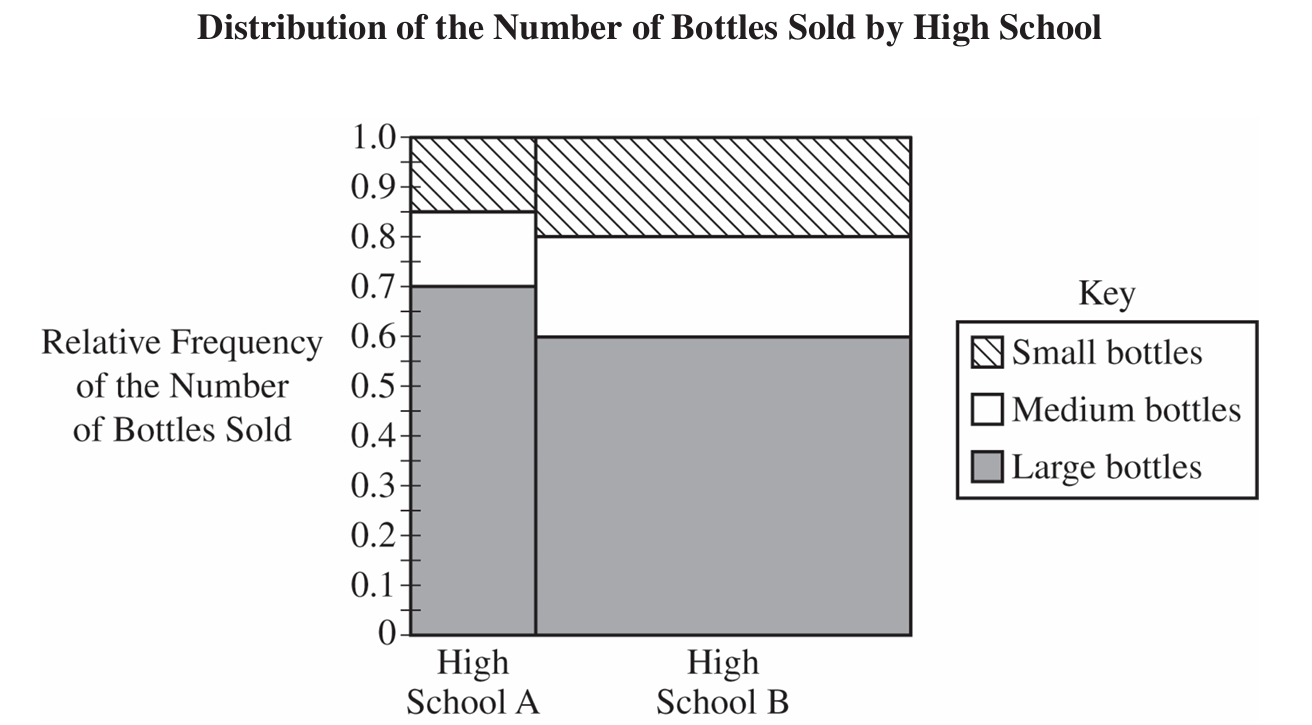
High School A sold a greater proportion of large bottles.
Looking at the y-axis of the mosaic plot, High School A’s proportion for large bottles is $0.7$, which is greater than High School B’s proportion of $0.6$.

(c)(ii)
High School B sold a greater number of large bottles.
In a mosaic plot, the total number of items is represented by the area of the segments.
Even though High School A had a larger proportion, the overall area of the rectangle representing large bottles for High School B is visibly larger than the area for High School A.

Question

To compare success rates for treating allergies at two clinics that specialize in treating allergy sufferers, researchers selected random samples of patient records from the two clinics. The following table summarizes the data.

(a) (i) Complete the following table by recording the relative frequencies of successful and unsuccessful treatments at each clinic.

(ii) Based on the relative frequency table in part (a-i), which clinic is more successful in treating allergy sufferers? Justify your answer.

(b) Based on the design of the study, would a statistically significant result allow the researchers to conclude that receiving treatments at the clinic you selected in part (a-ii) causes a higher percentage of successful treatments than at the other clinic? Explain your answer.

A physician who worked at both clinics believed that it was important to separate the patients in the study by severity of the patient’s allergy (severe or mild). The physician constructed the following mosaic plot. The values in the mosaic plot represent the number of patients who were either successfully treated or unsuccessfully treated in each allergy severity group within each clinic. For example, the value 78 represents the number of patients successfully treated in the mild group within Clinic A.

Based on the mosaic plot, the physician concluded the following:
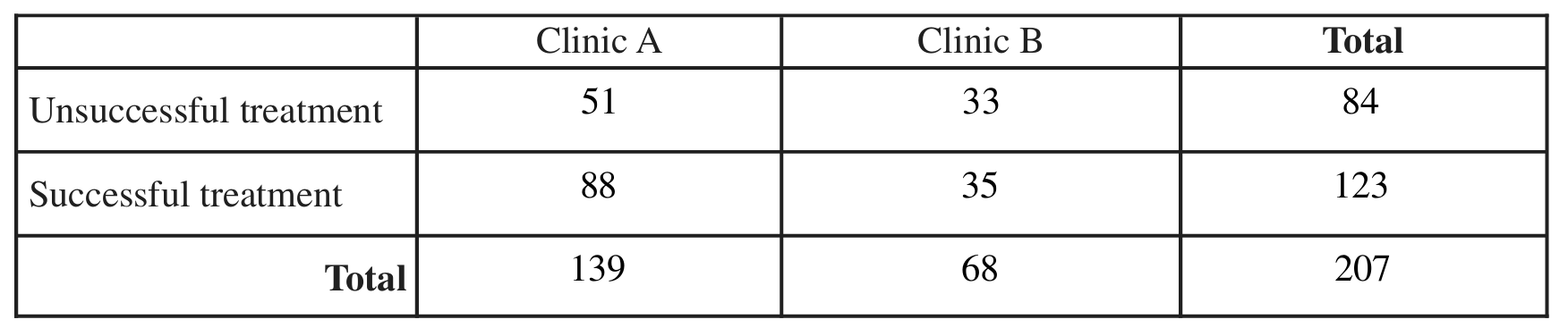
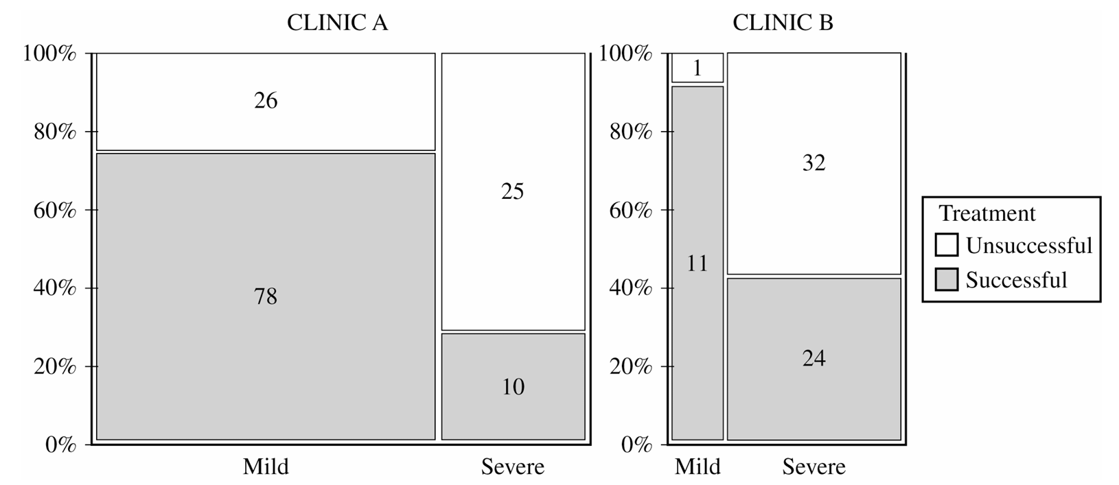
For mild allergy sufferers, Clinic B was more successful in treating allergies.
For severe allergy sufferers, Clinic B was more successful in treating allergies.

(c) (i) For each clinic, which allergy severity is treated more successfully? Justify your answer.

• Clinic A:
• Clinic B:

(ii) For each clinic, which allergy severity is more likely to be treated? Justify your answer.

• Clinic A:
• Clinic B:

(d) Using your answers from part (c), give a reasonable explanation of why the more successful clinic identified in part (a-ii) is the same as or different from the physician’s conclusion that Clinic B is more successful in treating both severe and mild allergies.

Most-appropriate topic codes (AP Statistics):

• Topic $1.10$ — The Investigative Question Revisited and Data Collection (Part $ \mathrm{b} $)
• Topic $2.1$ — Tabular and Graphical Representations for the Distributions of Two Categorical Variables (Parts $ \mathrm{a} $, $ \mathrm{c} $)
• Topic $2.2$ — Summary Statistics for Two Categorical Variables (Parts $ \mathrm{a} $, $ \mathrm{c} $, $ \mathrm{d} $)

▶️ Answer/Explanation

(a)(i)

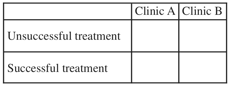
(a)(ii)
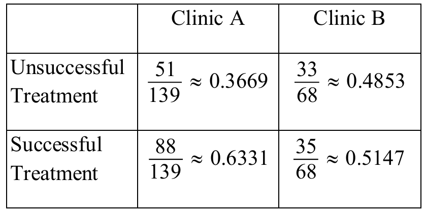
Clinic A is more successful. The relative frequency of successful treatments for Clinic A ($0.633$ or $63.3\%$) is greater than the relative frequency of successful treatments for Clinic B ($0.515$ or $51.5\%$).

(b)
No. The researchers selected random samples of patient records, which means this is an observational study, not a randomized experiment. Because patients were not randomly assigned to Clinic A or Clinic B, we cannot establish a cause-and-effect relationship due to the potential presence of confounding variables.

(c)(i)
• Clinic A: Mild allergies are treated more successfully. The success rate for mild is $78 / (78 + 26) = 75\%$, while the success rate for severe is $11 / (11 + 24) = 31.4\%$.
• Clinic B: Mild allergies are treated more successfully. The success rate for mild is $32 / (32 + 1) = 97\%$, while the success rate for severe is $10 / (10 + 25) = 28.6\%$.

(c)(ii)
• Clinic A: Mild allergies are more likely to be treated. Clinic A treated 104 mild cases ($78+26$) compared to only 35 severe cases ($11+24$).
• Clinic B: Severe allergies are more likely to be treated. Clinic B treated 35 severe cases ($10+25$) compared to only 33 mild cases ($32+1$).

(d)
The conclusion is different because of Simpson’s Paradox. Clinic A’s overall success rate is higher because it treats a much larger proportion of mild allergy cases, which naturally have a higher success rate regardless of the clinic. Conversely, Clinic B treats a higher proportion of severe cases, which brings its overall average down, even though it performs better than Clinic A within each specific severity group.

Question

A research center conducted a national survey about teenage behavior. Teens were asked whether they had consumed a soft drink in the past week. The following table shows the counts for three independent random samples from major cities.

(a) Suppose one teen is randomly selected from each city’s sample. A researcher claims that the likelihood of selecting a teen from Baltimore who consumed a soft drink in the past week is less than the likelihood of selecting a teen from either one of the other cities who consumed a soft drink in the past week because Baltimore has the least number of teens who consumed a soft drink. Is the researcher’s claim correct? Explain your answer.

(b) Consider the values in the table.

i. Construct a segmented bar chart of relative frequencies based on the information in the table.

ii. Which city had the smallest proportion of teens who consumed a soft drink in the previous week? Determine the value of the proportion.

(c) Consider the inference procedure that is appropriate for investigating whether there is a difference among the three cities in the proportion of all teens who consumed a soft drink in the past week.

i. Identify the appropriate inference procedure.
ii. Identify the hypotheses of the test.

Most-appropriate topic codes (AP Statistics):

• Topic $2.1$ — Tabular and Graphical Representations for the Distributions of Two Categorical Variables (Part $ \mathrm{b} $)
• Topic $2.2$ — Summary Statistics for Two Categorical Variables (Parts $ \mathrm{a} $, $ \mathrm{b} $)
• Topic $3.14$ — Setting Up a Chi-Square Test for Homogeneity or Independence (Part $ \mathrm{c} $)

▶️ Answer/Explanation

(a)
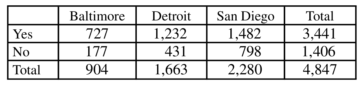
No, the researcher’s claim is incorrect because comparing mere counts is meaningless when the sample sizes across the cities are unequal. Instead, we must compare proportions: the proportion for Baltimore is $ \frac{727}{904} \approx 0.804 $, which is actually greater than the proportions for Detroit ($ \frac{1232}{1663} \approx 0.741 $) and San Diego ($ \frac{1482}{2280} = 0.65 $).

(b)(i)
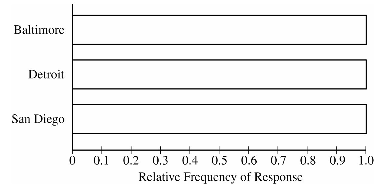
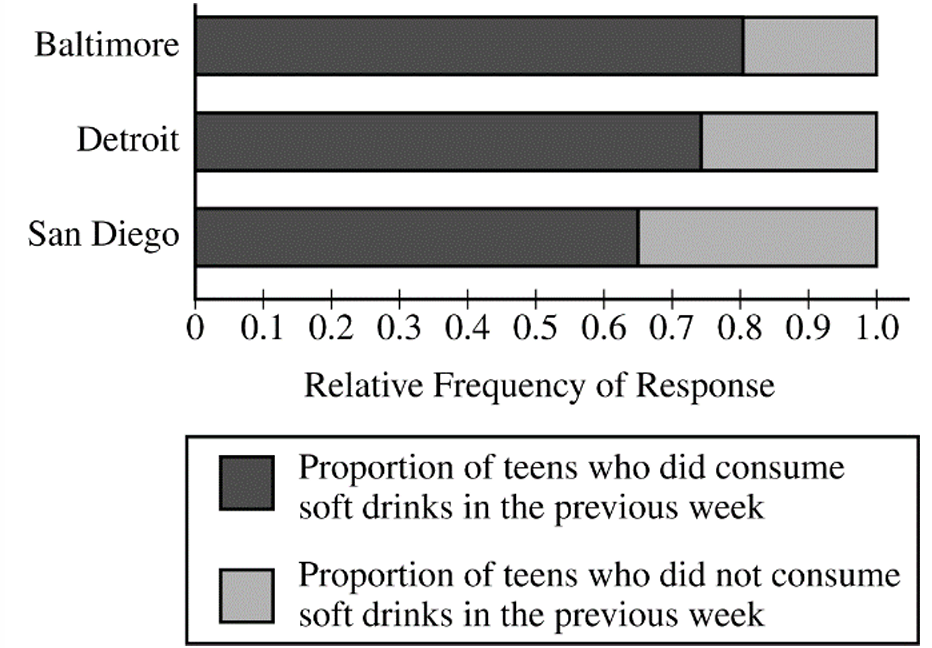
To construct the segmented bar chart, you would calculate the relative frequencies for “Yes” and “No” for each city and stack them so each bar reaches $1.0$ on the vertical axis. For example, Baltimore’s “Yes” segment would extend up to $ 0.804 $, with the “No” segment filling the rest up to $ 1.0 $.

(b)(ii)
San Diego had the smallest proportion of teens who consumed a soft drink, with a value of $ \frac{1482}{2280} = 0.65 $.

(c)(i)
A chi-square test for homogeneity is the appropriate inference procedure because we are investigating whether the distribution of a single categorical variable (consuming a soft drink) is the same across multiple independent populations (the three cities).

(c)(ii)
The null hypothesis $H_0$ is that there is no difference in the true proportion of all teens who consumed a soft drink in the past week across the three cities. The alternative hypothesis $H_a$ is that there is at least one difference in the proportion of all teens who consumed a soft drink in the past week across the three cities.

Question

A simple random sample of 100 high school seniors was selected from a large school district. The gender of each student was recorded, and each student was asked the following questions.

1. Have you ever had a part-time job?

2. If you answered yes to the previous question, was your part-time job in the summer only?

The responses are summarized in the table below.

(a) On the grid below, construct a graphical display that represents the association between gender and job experience for the students in the sample.

(b) Write a few sentences summarizing what the display in part (a) reveals about the association between gender and job experience for the students in the sample.

(c) Which test of significance should be used to test if there is an association between gender and job experience for the population of high school seniors in the district?

State the null and alternative hypotheses for the test, but do not perform the test.

Most-appropriate topic codes (AP Statistics):

• Topic $2.1$ — Tabular and Graphical Representations for the Distributions of Two Categorical Variables (Parts $\mathrm{a}$, $\mathrm{b}$)
• Topic $2.2$ — Summary Statistics for Two Categorical Variables (Part $\mathrm{b}$)
• Topic $3.14$ — Setting Up a Chi-Square Test for Homogeneity or Independence (Part $\mathrm{c}$)

▶️ Answer/Explanation

(a)
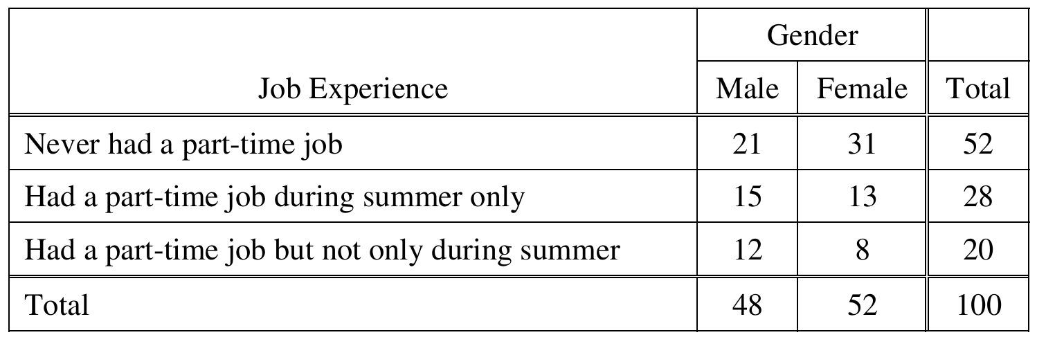
First, convert the raw counts to percentages within each gender so that males and females are directly comparable:
For Males $(n = 48)$:
• Never had a part-time job: $\dfrac{21}{48} \approx 43.8\%$
• Part-time job during summer only: $\dfrac{15}{48} \approx 31.2\%$
• Part-time job, not only during summer: $\dfrac{12}{48} = 25.0\%$
For Females $(n = 52)$:
• Never had a part-time job: $\dfrac{31}{52} \approx 59.6\%$
• Part-time job during summer only: $\dfrac{13}{52} = 25.0\%$
• Part-time job, not only during summer: $\dfrac{8}{52} \approx 15.4\%$

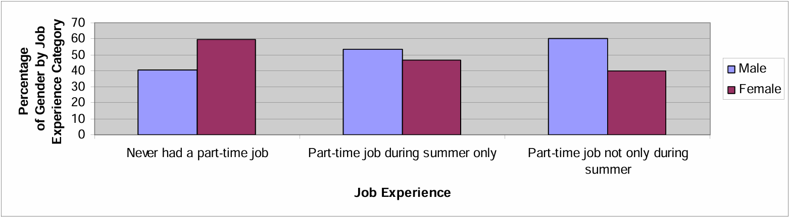
A side-by-side bar graph (or segmented bar graph) should be drawn with the three job-experience categories on the horizontal axis, percentage on the vertical axis, and separate bars (or segments) for Male and Female within each category. All axes must be labeled.

(b)
Looking at the bar graph, females were considerably more likely than males to have never had a part-time job — about $59.6\%$ of females compared with $43.8\%$ of males fall into that category.
On the other hand, males were more likely than females to have had a part-time job during the summer only ($31.2\%$ vs. $25.0\%$), and more likely to have had a part-time job that was not only during the summer ($25.0\%$ vs. $15.4\%$).
If there were no association between gender and job experience, we’d expect the bars for males and females to be roughly the same height in each category — but they clearly aren’t, so the sample data suggest there is an association between gender and job experience.

(c)
The appropriate test of significance is the chi-square test of association (or independence).
The chi-square test statistic is:
$ \chi^2 = \sum \frac{(\text{observed} – \text{expected})^2}{\text{expected}} $
The null and alternative hypotheses are:
$H_0$: There is no association between gender and job experience (for the population of high school seniors in the district).
$H_a$: There is an association between gender and job experience (for the population of high school seniors in the district).
Equivalently:
$H_0$: Gender and job experience are independent.
$H_a$: Gender and job experience are not independent.
Since we have two categorical variables each with multiple categories, the chi-square test of association/independence is the correct choice — a two-sample $z$-test for proportions only compares two groups on a binary outcome, and wouldn’t capture all three job-experience categories at once.

Question

A simple random sample of adults living in a suburb of a large city was selected. The age and annual income of each adult in the sample were recorded. The resulting data are summarized in the table below.

(a) What is the probability that a person chosen at random from those in this sample will be in the 31–45 age category?

(b) What is the probability that a person chosen at random from those in this sample whose incomes are over $\$50{,}000$ will be in the 31–45 age category? Show your work.

(c) Based on your answers to parts (a) and (b), is annual income independent of age category for those in this sample? Explain.

Most-appropriate topic codes (AP Statistics):

• Topic 2.1 — Tabular and Graphical Representations for the Distributions of Two Categorical Variables (All parts)
• Topic 2.6 — Conditional Probability (Part b)
• Topic 2.7 — Independent Events and Unions of Events (Part c)
• Topic 2.2 — Summary Statistics for Two Categorical Variables (Part a)

▶️ Answer/Explanation

(a)

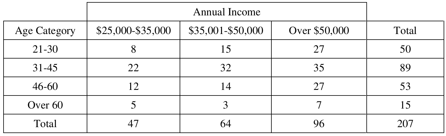
We want the probability that a randomly selected person from the sample falls in the 31–45 age category.
The total number of people in the sample is 207, and the number in the 31–45 age group is 89.
$ P(\text{age } 31\text{–}45) = \frac{89}{207} \approx 0.42995 $
$\boxed{P(\text{age } 31\text{–}45) \approx 0.4300}$

(b)

We now want the conditional probability that a person is in the 31–45 age category, given that their income is over $\$50{,}000$.
From the table, the total number of people with income over $\$50{,}000$ is 96, and among those, 35 are in the 31–45 age group.
$ P(\text{age } 31\text{–}45 \mid \text{income over } \$50{,}000) = \frac{35}{96} \approx 0.36458 $
$\boxed{P(\text{age } 31\text{–}45 \mid \text{income over } \$50{,}000) \approx 0.3646}$

(c)

For two variables to be independent, knowing the value of one variable should not change the probability of the other — in other words, the marginal probability and the conditional probability must be equal.
From part (a), $P(\text{age } 31\text{–}45) \approx 0.4300$, and from part (b), $P(\text{age } 31\text{–}45 \mid \text{income over } \$50{,}000) \approx 0.3646$.
Since these two probabilities are not equal ($0.4300 \neq 0.3646$), knowing a person’s income category does change the probability of being in the 31–45 age group.
Therefore, annual income and age category are not independent for those in this sample.

AP Statistics 2.2 Summary Statistics for Two Categorical Variables- Exam Style Questions - FRQs - New Syllabus

Question

Question

Question

Question

Question

Question

Resources

Members

Company