
AP Statistics 2.3 Estimating Probabilities Using Simulation- Exam Style Questions - FRQs - New Syllabus
Question

(ii) Calculate the proportion of bath fizzies that contain at least $\$10$.
Most-appropriate topic codes (AP Statistics):
• Topic \(2.8\) — Introduction to Random Variables and Probability Distributions (Part \( \mathrm{a} \))
• Topic \(2.9\) — Parameters of Random Variables (Parts \( \mathrm{c} \), \( \mathrm{d} \))
▶️ Answer/Explanation
(a) (i)
$P(X = 1) = 1 – (0.2 + 0.05 + 0.05 + 0.01 + 0.01)$
$P(X = 1) = 1 – 0.32$
$P(X = 1) = 0.68$
(a) (ii)
$P(X \ge 10) = P(X = 10) + P(X = 20) + P(X = 50) + P(X = 100)$
$P(X \ge 10) = 0.05 + 0.05 + 0.01 + 0.01$
$P(X \ge 10) = 0.12$
(b)
$P(X = 100 \mid X \ge 10) = \frac{P(X = 100 \text{ and } X \ge 10)}{P(X \ge 10)}$
$P(X = 100 \mid X \ge 10) = \frac{0.01}{0.12}$
$P(X = 100 \mid X \ge 10) \approx 0.0833 \text { or } \frac{1}{12} $
(c)
$E(X) = \sum [x \cdot P(x)]$
$E(X) = 1(0.68) + 5(0.2) + 10(0.05) + 20(0.05) + 50(0.01) + 100(0.01)$
$E(X) = 0.68 + 1 + 0.5 + 1 + 0.5 + 1$
$E(X) = \$4.68$
Interpretation: If many, many bath fizzies are randomly selected, the long-run average cash prize per fizzy will be approximately $\$4.68$.
(d)
$E(\text{euros}) = 0.89 \times E(X)$
$E(\text{euros}) = 0.89 \times 4.68$
$E(\text{euros}) \approx 4.1652 \text{ euros}$
Question
\(H_a : p_m – p_c < 0,\)
Most-appropriate topic codes (AP Statistics):
• Topic \(3.12\) — Setting Up a Test for the Difference Between Two Population Proportions (Part \( \mathrm{b} \))
• Topic \(3.13\) — Carrying Out a Test for the Difference Between Two Population Proportions (Part \( \mathrm{c} \))
• Topic \(2.3\) — Estimating Probabilities Using Simulation (Part \( \mathrm{c} \))
▶️ Answer/Explanation
(a)
No, it would not be reasonable to conclude that daily meditation causes a reduction in blood pressure. This study is an observational study — the men themselves chose whether or not to meditate; no treatment was randomly assigned. Because there was no randomization of treatment, cause-and-effect conclusions cannot be drawn from the results. Men who choose to meditate may differ from men who don’t in other important ways that are also related to blood pressure, such as being more health-conscious, exercising more, or having lower stress in general. These potential confounding variables make it impossible to isolate meditation as the cause.
(b)
For a normal approximation to be valid for the sampling distribution of \(\hat{p}_m – \hat{p}_c\), we need the number of successes and failures in each group to each be at least \(10\). First, compute the combined sample proportion of successes:
$\hat{p} = \frac{0 + 8}{11 + 17} = \frac{8}{28} \approx 0.286$
Then check each group:
For the meditation group \((n_m = 11)\):
$n_m \hat{p} = 11 \times \frac{8}{28} \approx 3.14 < 10 \quad \text{(condition fails)}$
For the non-meditation group \((n_c = 17)\):
$n_c \hat{p} = 17 \times \frac{8}{28} \approx 4.86 < 10 \quad \text{(condition fails)}$
Since the expected number of successes in both groups is less than \(10\), the normal approximation condition is not met, and it is not reasonable to use a normal approximation for the sampling distribution of \(\hat{p}_m – \hat{p}_c\).
(c)
First, compute the observed value of the sample statistic from the data:
$\hat{p}_m – \hat{p}_c = \frac{0}{11} – \frac{8}{17} \approx -0.47$
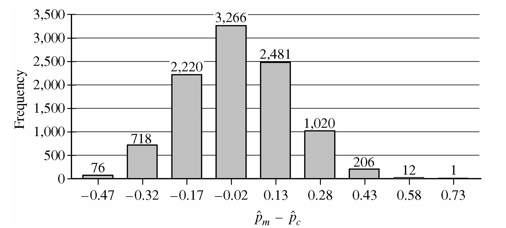
From the simulation histogram, only \(76\) out of \(10{,}000\) simulated values were \(-0.47\) or less (the most extreme negative outcome), giving an approximate \(p\)-value of:
$p\text{-value} \approx \frac{76}{10{,}000} = 0.0076$
Since this \(p\)-value of \(0.0076\) is very small (less than any common significance level such as \(\alpha = 0.05\)), we reject \(H_0\). There is convincing statistical evidence that men in this retirement community who meditate daily have a lower rate of high blood pressure than men who do not meditate. However, because this is an observational study, we can only conclude that meditation is associated with lower blood pressure — we cannot conclude that meditation causes a reduction in blood pressure.
Question


Most-appropriate topic codes (AP Statistics):
• Topic \(1.6\) — Descriptions for One Quantitative Variable Distributions (Part \(\mathrm{b}\))
• Topic \(2.3\) — Estimating Probabilities Using Simulation (Part \(\mathrm{c}\))
• Topic \(1.8\) — Graphical Representations of Summary Statistics for One Quantitative Variable (Part \(\mathrm{d}\))
▶️ Answer/Explanation
(a)
Let \(\mu\) = the true population mean fuel efficiency (in miles per gallon) for all cars of this particular model.
The consumer organization suspects the manufacturer is overstating the mpg, so the alternative hypothesis is lower-tailed:
\( H_0:\ \mu = 27\ \text{mpg} \)
\( H_a:\ \mu < 27\ \text{mpg} \)
The parameter must be defined as a population mean — not just a sample mean — and must be stated in context (fuel efficiency of this car model) to receive full credit.
(b)
Large values (greater than 1) of the ratio \(\dfrac{\text{sample mean}}{\text{sample median}}\) would indicate that the population distribution is skewed to the right.
The reason is that in a right-skewed distribution, the few unusually large values in the upper tail pull the mean upward, but the median — being a positional measure — is resistant to those extreme values and stays lower.
Therefore, when the distribution is right-skewed, we expect:
\( \text{sample mean} > \text{sample median} \implies \dfrac{\text{sample mean}}{\text{sample median}} > 1 \)
The further the ratio exceeds 1, the stronger the evidence of right-skewness.
(c)
The observed value of the statistic from the original sample is \(1.03\).
Looking at the dotplot of the 100 simulated statistics (all drawn from a normal population), we count that 14 out of 100 simulated values are greater than or equal to \(1.03\).
This gives a simulated \(p\)-value of approximately:
\( \hat{p} = \dfrac{14}{100} = 0.14 \)
Since \(0.14\) is larger than any commonly used significance level (such as \(\alpha = 0.05\) or \(\alpha = 0.10\)), we do not have convincing evidence that the original population is skewed to the right.
It is therefore plausible that the original sample of 10 cars came from a normally distributed population, and the observed right-skewness in the sample was simply due to random sampling variability.
(d)
Using only the five-number summary values, one reasonable skewness statistic is:
\( S = \dfrac{Q_3 – \text{Median}}{\text{Median} – Q_1} \)
Using the given data:
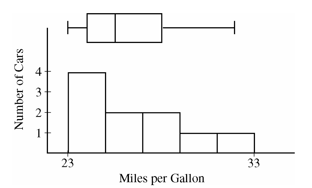
\( S = \dfrac{28 – 25.5}{25.5 – 24} = \dfrac{2.5}{1.5} \approx 1.67 \)
Values greater than 1 indicate right-skewness.
The reasoning is: in a right-skewed distribution, the data in the upper half are more spread out than in the lower half, so the distance from the median up to \(Q_3\) (the upper half of the middle 50%) will be larger than the distance from \(Q_1\) down to the median (the lower half of the middle 50%). This makes the numerator larger than the denominator, giving a ratio greater than 1.
Other acceptable statistics using only the five-number summary include:
\( S = \dfrac{\text{Maximum} – \text{Median}}{\text{Median} – \text{Minimum}}, \qquad S = \dfrac{\text{Maximum} – Q_3}{Q_1 – \text{Minimum}}, \qquad S = \dfrac{\frac{Q_1 + Q_3}{2}}{\text{Median}} \)
For all of these, values greater than 1 indicate right-skewness.
Question

Most-appropriate topic codes (AP Statistics):
• Topic \(4.5\) — Carrying Out a Test for a Population Mean or Population Mean Difference (Part \(\mathrm{a}\): test statistic, \(p\)-value, and conclusion)
• Topic \(2.3\) — Estimating Probabilities Using Simulation (Part \(\mathrm{b}\): simulation-based estimation of a \(p\)-value)
• Topic \(3.6\) — p-Values (Part \(\mathrm{b}\): interpreting simulated \(p\)-value evidence)
▶️ Answer/Explanation
(a)
Let \(\mu\) = the true mean number of fluid ounces dispensed into all juice bottles filled by the machine in the past hour.
Step 1 — Hypotheses:
\(H_0: \mu = 12.1\)
\(H_a: \mu \neq 12.1\)
Step 2 — Test: One-sample \(t\)-test for a mean (conditions are given as met; population standard deviation is unknown).
\(t = \frac{\bar{x} – \mu_0}{s/\sqrt{n}}\)
Step 3 — Mechanics:
Given: \(\bar{x} = 12.05\), \(s = 0.085\), \(n = 4\), \(\mu_0 = 12.1\)
\(t = \frac{12.05 – 12.1}{0.085/\sqrt{4}} = \frac{-0.05}{0.0425} \approx -1.176\)
Degrees of freedom: \(df = n – 1 = 3\)
Two-sided \(p\)-value:
\(p\text{-value} = 2 \cdot P(T_3 < -1.176) \approx 0.324\)
Step 4 — Conclusion:
Since the \(p\)-value of \(0.324\) is much larger than any reasonable significance level (such as \(\alpha = 0.05\)), we fail to reject \(H_0\).
There is not sufficient evidence to conclude that the mean amount of juice being dispensed is different from \(12.1\) fluid ounces. The machine does not need to be shut down on the basis of the mean.
(b)
In the simulation, 300 samples of size 4 were drawn from a normal population with \(\sigma = 0.05\). The sample standard deviation of \(s = 0.085\) from our actual data falls well out in the right tail of the dotplot.
Counting the dots at or beyond \(0.085\) in the dotplot, only about 12 out of 300 simulated values are as large or larger than \(0.085\).
This gives an estimated (simulated) \(p\)-value of:
\(\hat{p}\text{-value} = \frac{12}{300} = 0.04\)
Since this simulated \(p\)-value of \(0.04\) is less than \(\alpha = 0.05\), the sample does provide convincing evidence that the true standard deviation of the juice dispensed exceeds \(0.05\) fluid ounce. The machine should be shut down for recalibration.
Question
| Sample | Minimum | Sample | Minimum | Sample | Minimum |
| 1 | 121.45 | 51 | 124.28 | 101 | 125.25 |
| 2 | 122.51 | 52 | 124.29 | 102 | 125.31 |
| 3 | 122.53 | 53 | 124.30 | 103 | 125.36 |
| 4 | 122.72 | 54 | 124.31 | 104 | 125.38 |
| 5 | 122.75 | 55 | 124.34 | 105 | 125.40 |
| 6 | 122.89 | 56 | 124.36 | 106 | 125.42 |
| 7 | 122.93 | 57 | 124.37 | 107 | 125.48 |
| 8 | 122.99 | 58 | 124.37 | 108 | 125.49 |
| 9 | 123.04 | 59 | 124.39 | 109 | 125.50 |
| 10 | 123.08 | 60 | 124.39 | 110 | 125.52 |
| 11 | 123.09 | 61 | 124.41 | 111 | 125.54 |
| 12 | 123.10 | 62 | 124.44 | 112 | 125.56 |
| 13 | 123.31 | 63 | 124.53 | 113 | 125.61 |
| 14 | 123.34 | 64 | 124.53 | 114 | 125.67 |
| 15 | 123.39 | 65 | 124.54 | 115 | 125.72 |
| 16 | 123.40 | 66 | 124.55 | 116 | 125.76 |
| 17 | 123.41 | 67 | 124.55 | 117 | 125.77 |
| 18 | 123.41 | 68 | 124.55 | 118 | 125.78 |
| 19 | 123.46 | 69 | 124.55 | 119 | 125.79 |
| 20 | 123.49 | 70 | 124.58 | 120 | 125.84 |
| 21 | 123.51 | 71 | 124.67 | 121 | 125.87 |
| 22 | 123.57 | 72 | 124.69 | 122 | 125.87 |
| 23 | 123.58 | 73 | 124.73 | 123 | 125.90 |
| 24 | 123.59 | 74 | 124.77 | 124 | 125.90 |
| 25 | 123.60 | 75 | 124.78 | 125 | 125.93 |
| 26 | 123.66 | 76 | 124.78 | 126 | 125.93 |
| 27 | 123.67 | 77 | 124.80 | 127 | 125.93 |
| 28 | 123.72 | 78 | 124.80 | 128 | 125.94 |
| 29 | 123.75 | 79 | 124.81 | 129 | 125.98 |
| 30 | 123.77 | 80 | 124.85 | 130 | 126.00 |
| 31 | 123.78 | 81 | 124.91 | 131 | 126.03 |
| 32 | 123.84 | 82 | 124.92 | 132 | 126.05 |
| 33 | 123.91 | 83 | 124.92 | 133 | 126.05 |
| 34 | 123.93 | 84 | 124.96 | 134 | 126.06 |
| 35 | 123.95 | 85 | 125.00 | 135 | 126.09 |
| 36 | 123.95 | 86 | 125.01 | 136 | 126.15 |
| 37 | 123.98 | 87 | 125.02 | 137 | 126.15 |
| 38 | 123.99 | 88 | 125.02 | 138 | 126.16 |
| 39 | 124.05 | 89 | 125.03 | 139 | 126.19 |
| 40 | 124.05 | 90 | 125.04 | 140 | 126.19 |
| 41 | 124.06 | 91 | 125.05 | 141 | 126.25 |
| 42 | 124.12 | 92 | 125.07 | 142 | 126.26 |
| 43 | 124.14 | 93 | 125.08 | 143 | 126.33 |
| 44 | 124.15 | 94 | 125.09 | 144 | 126.35 |
| 45 | 124.16 | 95 | 125.14 | 145 | 126.45 |
| 46 | 124.19 | 96 | 125.18 | 146 | 126.50 |
| 47 | 124.23 | 97 | 125.21 | 147 | 126.57 |
| 48 | 124.27 | 98 | 125.21 | 148 | 126.62 |
| 49 | 124.28 | 99 | 125.22 | 149 | 126.64 |
| 50 | 124.28 | 100 | 125.25 | 150 | 126.95 |
Most-appropriate topic codes (AP Statistics):
• Topic 4.5 — Carrying Out a Test for a Population Mean or Population Mean Difference (Part a)
• Topic 2.11 — The Normal Distribution (Parts b, c)
• Topic 2.3 — Estimating Probabilities Using Simulation (Part d)
▶️ Answer/Explanation
(a)
Step 1 — State the hypotheses:
\( H_0: \mu = 128 \text{ fl oz} \quad \text{vs.} \quad H_a: \mu < 128 \text{ fl oz} \)
where \(\mu\) is the true mean amount of milk in containers from this plant.
We test whether the mean is below 128 fl oz, since that would indicate non-compliance.
Step 2 — Identify the procedure and check conditions:
Use a one-sample \(t\)-test for a mean:
\( t = \frac{\bar{x} – \mu_0}{s/\sqrt{n}} \)
The problem states the filling process produces a normal distribution, so the normality condition is satisfied.
The containers were randomly sampled, so independence holds.
Step 3 — Compute the test statistic and p-value:
With \(\bar{x} = 127.2\), \(\mu_0 = 128\), \(s = 2.1\), \(n = 12\):
\( t = \frac{127.2 – 128}{2.1/\sqrt{12}} = \frac{-0.8}{0.6062} \approx -1.319 \)
Degrees of freedom: \(df = n – 1 = 11\).
For a one-tailed test with \(t = -1.319\) and \(df = 11\):
\( p\text{-value} = P(T_{11} < -1.319) \approx 0.107 \)
Step 4 — State the conclusion in context:
Since the p-value of \(0.107\) is greater than any reasonable significance level (e.g., \(\alpha = 0.05\)), we fail to reject \(H_0\). There is not sufficient evidence to conclude that the plant is out of compliance. The sample mean of 127.2 fl oz is below 128, but the difference is small enough that it could plausibly be due to random sampling variability alone.
(b)
Let \(X\) be the amount of milk in a randomly selected container, where \(X \sim N(128.0,\ 2.0)\). We want \(P(X \geq 125)\).
Standardize by converting to a \(z\)-score: \( z = \frac{125 – 128}{2} = \frac{-3}{2} = -1.5 \)
Using the standard normal table:
\( P(X \geq 125) = P(Z \geq -1.5) = 1 – P(Z < -1.5) = 1 – 0.0668 \)
\( \boxed{P(X \geq 125) = 0.9332} \)
So about 93.3% of containers from this machine will contain at least 125 fl oz.
(c)
Let \(X_{(1)} = \min(X_1, X_2, \ldots, X_{12})\) be the smallest value among 12 randomly selected containers.
For the minimum to be at least 125 fl oz, every single one of the 12 containers must contain at least 125 fl oz.
Since the containers are independent:
\( P(X_{(1)} \geq 125) = P(X_1 \geq 125) \times P(X_2 \geq 125) \times \cdots \times P(X_{12} \geq 125) \)
\( = [P(X \geq 125)]^{12} = (0.9332)^{12} \)
\( \boxed{P(X_{(1)} \geq 125) \approx 0.4362} \)
There is roughly a 43.6% chance that the smallest of 12 containers all meet the 125 fl oz threshold.
Even though each individual container has a 93.3% chance of passing, the probability that all 12 pass simultaneously drops considerably.
(d)
From the sorted list of 150 simulated minimums, we count how many are at least 125 fl oz. Scanning the table, the minimums first reach 125.00 at sample 85. From sample 85 through sample 150, that gives:
\( 150 – 85 + 1 = 66 \text{ minimums that are} \geq 125 \text{ fl oz} \)
The simulated probability estimate is therefore:
\( \hat{p} = \frac{66}{150} \approx \boxed{0.44} \)
Comparison with the theoretical value:
The theoretical probability from part (c) was \(0.4362\).
The simulation estimate of \(0.44\) is very close — the difference is only:
\( |0.44 – 0.4362| = 0.0038 \)
This is a tiny discrepancy, which is exactly what we expect from a simulation of this size.
The simulation does an excellent job of approximating the true theoretical probability, confirming that the independence-based calculation in part (c) is correct.
Question
Most-appropriate topic codes (AP Statistics):
• Topic 2.7 — Independent Events and Unions of Events (Part a,b)
• Topic 2.4 — Introduction to Probability (Part b)
• Topic 2.3 — Estimating Probabilities Using Simulation (Part c)
•Topic 1.12 — Potential Problems with Sampling (Part d)
▶️ Answer/Explanation
(a)
The probability distribution of \(X\) is not binomial because the bones are selected without replacement from a finite population of only 20 femurs. For a binomial distribution to apply, each trial must be independent — that is, the probability of success (selecting a male femur) must remain constant from one draw to the next. However, when sampling without replacement, the composition of the remaining pool changes with each selection, so the probability of drawing a male femur on each successive draw depends on what was drawn before it. Since the trials are not independent and the probability of success is not fixed, the distribution of \(X\) is hypergeometric, not binomial.
\(\boxed{X \text{ is not binomial because sampling is without replacement, making trials dependent}}\)
(b)
With 10 males and 10 females among the 20 brontosaurs, compute the probability that all 4 selected femurs are male using the multiplication rule for dependent events (without replacement):
\(P(\text{1st is male}) = \dfrac{10}{20}\)
\(P(\text{2nd is male} \mid \text{1st is male}) = \dfrac{9}{19}\)
\(P(\text{3rd is male} \mid \text{first two are male}) = \dfrac{8}{18}\)
\(P(\text{4th is male} \mid \text{first three are male}) = \dfrac{7}{17}\)
Therefore:
\(P(\text{all 4 are male}) = \dfrac{10}{20} \times \dfrac{9}{19} \times \dfrac{8}{18} \times \dfrac{7}{17}\)
\(= \dfrac{10 \times 9 \times 8 \times 7}{20 \times 19 \times 18 \times 17} = \dfrac{5040}{116280} \approx 0.0433\)
This can also be expressed using combinations:
\(P(\text{all 4 are male}) = \dfrac{\dbinom{10}{4}}{\dbinom{20}{4}} = \dfrac{210}{4845} \approx 0.0433\)
\(\boxed{P(\text{all 4 male}) \approx 0.0433}\)
(c)
No, it does not seem likely that males and females were equally represented in the group of 20 brontosaurs. From part (b), if the group had exactly 10 males and 10 females, the probability of randomly selecting 4 males in a row is only about \(4.33\%\). Since this probability is quite small (less than 5%), observing all 4 selected femurs being male is an unusual result under the assumption of equal representation. It is therefore more reasonable to think that males outnumbered females in this particular group of brontosaurs trapped in the swamp, though equal representation is possible — just unlikely given the data.
\(\boxed{\text{Equal representation is unlikely; evidence suggests more males than females in the group}}\)
(d)
No, it is not reasonable to generalize the conclusion from part (c) to the entire population of brontosaurs. The 20 brontosaurs found at the site do not constitute a random sample from the population of all brontosaurs — they represent only those individuals that happened to wander into that particular swamp and become trapped. This is a highly specific and non-random group. It is plausible that behavioral differences between male and female brontosaurs (for example, males may have been more likely to venture into deep swamp areas while foraging) could explain why males are overrepresented in this particular site. Such a non-representative sample cannot be used to draw conclusions about the broader population of all brontosaurs.
\(\boxed{\text{Cannot generalize; the 20 brontosaurs are not a random sample of all brontosaurs}}\)