
AP Statistics 2.6 Conditional Probability- Exam Style Questions - FRQs - New Syllabus
Question

Most-appropriate topic codes (AP Statistics):
• Topic \(2.7\) — Independent Events and Mutually Exclusive Events (Part \( \mathrm{b} \))
• Topic \(2.10\) — The Binomial Distribution (Part \( \mathrm{c} \))
▶️ Answer/Explanation
(a)(i)
From the given two-way table, we can find the joint probability directly by looking at the intersection of the “Women” row and “Never” column.
\(P(\text{never and woman}) = 0.0636\)
(a)(ii)
To find this probability, we use the general addition rule by adding the marginal probability of “never” to the marginal probability of “woman”, and subtracting their intersection.
\(P(\text{never or woman}) = P(\text{never}) + P(\text{woman}) – P(\text{never and woman})\)
\(P(\text{never or woman}) = 0.1200 + 0.5300 – 0.0636 = 0.5864\)
(a)(iii)
For conditional probability, we divide the joint probability of both events occurring by the marginal probability of the given condition (“woman”).
\(P(\text{never} \mid \text{woman}) = \dfrac{P(\text{never and woman})}{P(\text{woman})}\)
\(P(\text{never} \mid \text{woman}) = \dfrac{0.0636}{0.5300} = 0.12\)
(b)
We can check for independence by seeing if the conditional probability of an event equals its marginal probability.
Since \(P(\text{never} \mid \text{woman}) = 0.12\) and the overall probability \(P(\text{never}) = 0.12\), the probabilities are identical.
Yes, this indicates that the event of responding “never” is perfectly independent of the event of being a “woman”.
(c)
This scenario can be modeled using a binomial distribution with \(n=5\) trials and a success probability of \(p=0.54\).
We need to find the probability of getting at least \(4\) successes, which means finding the sum of \(P(X=4)\) and \(P(X=5)\).
\(P(X \ge 4) = \binom{5}{4}(0.54)^4(0.46)^1 + \binom{5}{5}(0.54)^5(0.46)^0\)
\(P(X \ge 4) \approx 0.19557 + 0.04592 \approx 0.24149\)
Question
If heads, you must respond no, regardless of whether you regularly recycle. If tails, please truthfully respond yes or no.
Most-appropriate topic codes (AP Statistics):
• Topic \(2.6\) — Conditional Probability (Part \( \mathrm{c}\text{-}\mathrm{ii} \))
• Topic \(2.8\) — Introduction to Random Variables and Probability Distributions (Part \( \mathrm{c}\text{-}\mathrm{i} \))
• Topic \(3.3\) — Constructing a Confidence Interval for a Population Proportion (Part \( \mathrm{a} \))
▶️ Answer/Explanation
(a)
The sample selected by the environmental science teacher contained $60$ students.
Detailed Solution:
First, find the point estimate $\hat{p}$ which is the midpoint of the confidence interval: $\hat{p} = \frac{0.584 + 0.816}{2} = 0.70$.
Next, determine the margin of error ($ME$) by calculating the distance from the midpoint to an endpoint: $ME = 0.816 – 0.70 = 0.116$.
Using the margin of error formula $ME = z^* \sqrt{\frac{\hat{p}(1-\hat{p})}{n}}$ for a $95\%$ confidence level ($z^* = 1.96$), we set up the equation $0.116 = 1.96 \sqrt{\frac{0.70(1-0.70)}{n}}$.
Solving for $n$ gives us $\sqrt{n} = \frac{1.96 \sqrt{0.21}}{0.116} \approx 7.74$, which squares to $n \approx 59.9$, revealing that the teacher’s sample size is exactly $60$ students.
(b)
Bias might have been introduced because students were asked directly by their environmental science teacher, which likely creates response bias.
Detailed Solution:
Because the survey is conducted face-to-face by a teacher who is expected to care about the environment, students may feel strong social pressure to give the “desirable” answer.
This phenomenon is known as response bias, where respondents do not answer truthfully in order to avoid judgment or please the interviewer.
As a result, more students will claim they recycle than actually do, artificially inflating the number of “yes” responses and causing the point estimate to be higher than the true population proportion.
(c)(i)
The expected number of students required to respond “no” due to the coin flip is $150$.
Detailed Solution:
Since the students are flipping a fair coin, the theoretical probability of getting heads is exactly $0.5$.
With a total random sample of $n = 300$ students, the expected number of heads is calculated as $n \times p = 300 \times 0.5$.
Therefore, we can expect exactly half the students, or $150$, to be forced to respond “no” based on the coin flip instructions.
(c)(ii)
The point estimate for the proportion of all students at the high school who would respond “yes” is $0.58$.
Detailed Solution:
Out of the $300$ total students, $213$ responded “no”, and we expect $150$ of these “no” responses to come from the students who flipped heads.
This means the remaining $213 – 150 = 63$ “no” responses came from the $150$ students who flipped tails and answered truthfully about not recycling.
Since $150$ students flipped tails and $63$ of them truthfully said “no”, the remaining $150 – 63 = 87$ students must have truthfully answered “yes”.
Thus, the point estimate for the proportion of students who actually recycle is $\frac{87}{150} = 0.58$.
Question
Most-appropriate topic codes (AP Statistics):
• Topic \(2.7\) — Independent Events and Mutually Exclusive Events (Parts \( \mathrm{a} \), \( \mathrm{b} \))
• Topic \(2.10\) — The Binomial Distribution (Part \( \mathrm{c} \))
▶️ Answer/Explanation
(a)
Let \(L\) denote the event that a child is left-handed, \(M\) denote the event of a multiple birth, and \(S\) denote the event of a single birth.
We are given: \(P(M) = 0.035\), \(P(S) = 0.965\), \(P(L \mid M) = 0.22\), and \(P(L \mid S) = 0.11\).
Apply the Law of Total Probability:
\(P(L) = P(M) \cdot P(L \mid M) + P(S) \cdot P(L \mid S)\)
\(P(L) = (0.035)(0.22) + (0.965)(0.11)\)
\(P(L) = 0.0077 + 0.10615\)
\(\boxed{P(L) = 0.11385}\)
Think of this as a weighted average of the two left-handedness rates — you weight each group’s rate by how large that group is. Since single births make up the overwhelming majority (96.5%), they drive the overall rate, which lands very close to 11%. The small multiple-birth group nudges it up just slightly to about 11.4%.
(b)
We use the definition of conditional probability to find \(P(M \mid L)\).
\(P(M \mid L) = \dfrac{P(M \cap L)}{P(L)}\)
The joint probability \(P(M \cap L)\) is found using the multiplication rule:
\(P(M \cap L) = P(M) \cdot P(L \mid M) = (0.035)(0.22) = 0.0077\)
Using \(P(L) = 0.11385\) from part (a):
\(P(M \mid L) = \dfrac{0.0077}{0.11385}\)
\(\boxed{P(M \mid L) \approx 0.0676}\)
This is a classic Bayes-style reversal — we flipped from “given multiple birth, what’s the chance of being left-handed?” to “given left-handed, what’s the chance of multiple birth?” Even though multiple-birth children are twice as likely to be left-handed (22% vs. 11%), they are so rare (only 3.5% of all births) that among all left-handed children, only about 6.8% actually come from multiple births. Rarity wins.
(c)
Let \(X\) represent the number of left-handed children in a random sample of \(20\). Since each child is selected independently with the same probability of being left-handed, \(X\) follows a binomial distribution:
\(X \sim \operatorname{Binomial}(n = 20,\; p = 0.11385)\)
We want \(P(X \geq 3)\). Using the complement:
\(P(X \geq 3) = 1 – P(X \leq 2) = 1 – \bigl[P(X = 0) + P(X = 1) + P(X = 2)\bigr]\)
Using the binomial formula \(\displaystyle P(X = k) = \binom{20}{k}(0.11385)^{k}(0.88615)^{20-k}\):
\(P(X = 0) = \dbinom{20}{0}(0.11385)^{0}(0.88615)^{20} \approx 0.0891\)
\(P(X = 1) = \dbinom{20}{1}(0.11385)^{1}(0.88615)^{19} \approx 0.2289\)
\(P(X = 2) = \dbinom{20}{2}(0.11385)^{2}(0.88615)^{18} \approx 0.2797\)
Summing the complement terms:
\(P(X \leq 2) \approx 0.0891 + 0.2289 + 0.2797 = 0.5977\)
\(P(X \geq 3) = 1 – 0.5977\)
\(\boxed{P(X \geq 3) \approx 0.402}\)
The complement trick is your best friend here — instead of adding up \(P(X=3) + P(X=4) + \cdots + P(X=20)\), which would take forever, you subtract the small pile of easy cases (0, 1, or 2 left-handed kids) from 1. With only about an 11.4% chance per child, there’s roughly a 40% chance that 3 or more kids in a group of 20 will be left-handed — higher than you might expect, because “at least 3” covers most of the distribution.
Question
Most-appropriate topic codes (AP Statistics):
• Topic \(2.7\) — Independent Events and Mutually Exclusive Events (Parts \( \mathrm{b} \), \( \mathrm{c} \))
• Topic \(2.11\) — The Normal Distribution (Part \( \mathrm{a} \))
▶️ Answer/Explanation
(a)
Let \(X\) denote the diameter (in mm) of a randomly selected melon from Distributor J. We are told that \(X\) follows an approximately normal distribution with mean \(\mu = 133\) mm and standard deviation \(\sigma = 5\) mm.
First, convert the boundary value to a \(z\)-score:
\( z = \dfrac{137 – 133}{5} = \dfrac{4}{5} = 0.8 \)
Now find the probability to the right of \(z = 0.8\) using the standard normal table:
\( P(X > 137) = P(Z > 0.8) = 1 – P(Z < 0.8) = 1 – 0.7881 \)
\( \boxed{P(X > 137) = 0.2119} \)
(b)
Define the following events:
\(J\): the melon is from Distributor J
\(K\): the melon is from Distributor K
\(G\): the melon has a diameter greater than \(137\) mm
We are given \(P(J) = 0.70\), \(P(K) = 0.30\), \(P(G \mid J) = 0.2119\), and \(P(G \mid K) = 0.8413\).
Using the Law of Total Probability:
\( P(G) = P(G \mid J)\cdot P(J) + P(G \mid K)\cdot P(K) \)
\( P(G) = (0.2119)(0.70) + (0.8413)(0.30) \)
\( P(G) = 0.14833 + 0.25239 \)
\( \boxed{P(G) = 0.4007} \)
(c)
We want the conditional probability that the melon is from Distributor J, given that its diameter is greater than \(137\) mm. Using the definition of conditional probability:
\( P(J \mid G) = \dfrac{P(J \cap G)}{P(G)} \)
The joint probability \(P(J \cap G)\) was found in part (b):
\( P(J \cap G) = P(G \mid J)\cdot P(J) = (0.2119)(0.70) = 0.14833 \)
Substituting into the formula:
\( P(J \mid G) = \dfrac{0.14833}{0.40072} \)
\( \boxed{P(J \mid G) \approx 0.3701} \)
Even though Distributor J supplies \(70\%\) of the melons in the store, only about \(37\%\) of the large-diameter melons (over \(137\) mm) come from Distributor J — this makes sense because Distributor K’s melons are much more likely to be large, so they dominate that group despite being the smaller supplier.
Question
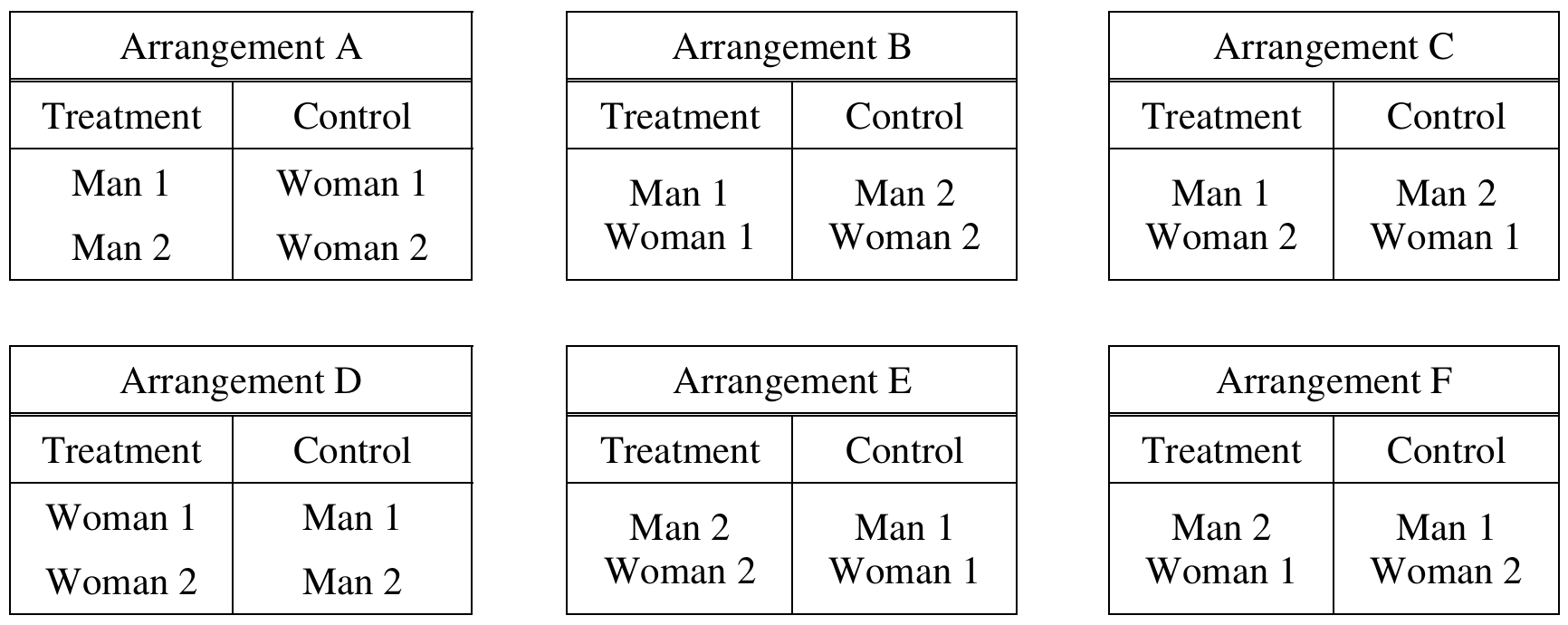
(i) Complete the table below by calculating the probability of each arrangement occurring if the sequential coin flip method is used.

(i) Complete the table below by calculating the probability of each arrangement occurring if the chip method is used.
Most-appropriate topic codes (AP Statistics):
• Topic \(2.6\) — Conditional Probability (Parts \( \mathrm{a} \), \( \mathrm{b} \))
• Topic \(2.7\) — Independent Events and Mutually Exclusive Events (Parts \( \mathrm{a} \), \( \mathrm{b} \))
▶️ Answer/Explanation
(a)(i)
Let T (tail) represent being assigned to the treatment group and H (head) represent being assigned to the control group. The process stops as soon as one group fills up. We trace each possible sequence of flips:

(a)(ii)
Man 1 and Man 2 are assigned to the same group only in Arrangements A (both in treatment) and D (both in control). So the probability is:
\(P(A) + P(D) = \dfrac{1}{4} + \dfrac{1}{4} = \boxed{\dfrac{1}{2}}\)
(b)(i)
Let T represent being assigned to the treatment group and C represent being assigned to the control group. Since chips are drawn without replacement from a pool of 2 T chips and 2 C chips, the probabilities change at each draw. Working through each arrangement:

(b)(ii)
Man 1 and Man 2 are in the same group only in Arrangements A and D. Therefore:
\(P(A) + P(D) = \dfrac{1}{6} + \dfrac{1}{6} = \boxed{\dfrac{1}{3}}\)
(c)
The chip method should be used. Here is the reasoning:
From parts (a)(i) and (b)(i), the chip method gives every arrangement an equal probability of \(\dfrac{1}{6}\), while the coin flip method assigns unequal probabilities — arrangements A and D each have probability \(\dfrac{1}{4}\), while B, C, E, and F each have probability \(\dfrac{1}{8}\).
From parts (a)(ii) and (b)(ii), the probability that both men end up in the same group is \(\dfrac{1}{2}\) under the coin method but only \(\dfrac{1}{3}\) under the chip method. Since students enter first and teachers enter next, the coin flip method is more likely to place all students together in one group — if teachers and students have different food preferences, this imbalance would make it impossible to tell whether any observed difference in lunch preference is due to the treatment (type of lunch) or the role of the participant (teacher vs. student).
The chip method, by giving all arrangements an equal chance, is therefore more appropriate for this experiment.
Question
Most-appropriate topic codes (AP Statistics):
• Topic \(2.7\) — Independent Events and Unions of Events (Parts \( \mathrm{a} \), \( \mathrm{b} \))
• Topic \(3.6\) — \(p\)-Values (Part \( \mathrm{c} \))
▶️ Answer/Explanation
(a)
Since failures are independent and the failure rate is \(p = 0.15\), the probability that a single super igniter successfully launches a rocket is:
\(P(\text{success}) = 1 – 0.15 = 0.85\)
For the first 30 super igniters to all successfully launch, each of the 30 independent trials must be a success:
\(P(\text{first 30 all succeed}) = (0.85)^{30}\)
\(P(\text{first 30 all succeed}) = (0.85)^{30} \approx 0.0076\)
\(\boxed{P \approx 0.0076}\)
(b)
We are told the first 30 igniters all succeeded. We want the probability that the first failure occurs on either the 31st or the 32nd igniter tested.
For the first failure to occur on the 31st igniter, the 31st must fail. Since failures are independent and we are conditioning on the 30 prior successes:
\(P(\text{failure on 31st}) = 0.15\)
For the first failure to occur on the 32nd igniter, the 31st must succeed AND the 32nd must fail:
\(P(\text{failure on 32nd}) = (0.85)(0.15) = 0.1275\)
These two events are mutually exclusive, so:
\(P(\text{first failure on 31st or 32nd}) = 0.15 + (0.85)(0.15)\)
\(= 0.15 + 0.1275 = 0.2775\)
\(\boxed{P \approx 0.2775}\)
(c)
Yes, it is reasonable to believe that the failure rate of the super igniters is less than 15 percent.
If the failure rate were truly 15 percent (same as the original igniters), the probability of the first 30 super igniters all successfully launching rockets would be only about \(0.0076\), or less than 1 percent. This is an extremely unlikely outcome under the assumption that the failure rate is 15 percent.
Because observing 30 consecutive successes would be so rare if the failure rate were really 15 percent, getting this result in the test provides strong evidence that the true failure rate of the super igniters is lower than 15 percent. The data are inconsistent with a 15 percent failure rate, so it is indeed reasonable to believe the super igniters have a lower failure rate than the original igniters.
Question

Most-appropriate topic codes (AP Statistics):
• Topic \(2.8\) — Introduction to Random Variables and Probability Distributions (Part \( \mathrm{a} \))
• Topic \(2.9\) — Parameters of Random Variables (Parts \( \mathrm{b} \), \( \mathrm{d} \))
▶️ Answer/Explanation
(a)
The probability that at least one ATM is working when the mall opens is the sum of the probabilities for \(1\), \(2\), and \(3\) ATMs.
\( P(X \ge 1) = 0.21 + 0.40 + 0.24 \)
\( P(X \ge 1) = 0.85 \)
(b)
The expected value of the number of ATMs that are working when the mall opens is found by multiplying each possible value by its corresponding probability and summing the results.
\( E(X) = 0(0.15) + 1(0.21) + 2(0.40) + 3(0.24) \)
\( E(X) = 0 + 0.21 + 0.80 + 0.72 \)
\( E(X) = 1.73 \text{ machines} \)
(c)
The probability that all three ATMs are working given that at least one ATM is working is calculated using the conditional probability formula.
\( P(X=3 \mid X \ge 1) = \dfrac{P(X=3 \text{ and } X \ge 1)}{P(X \ge 1)} \)
\( P(X=3 \mid X \ge 1) = \dfrac{P(X=3)}{P(X \ge 1)} \)
\( P(X=3 \mid X \ge 1) = \dfrac{0.24}{0.85} \approx 0.282 \)
(d)
Given that at least one ATM is working, the expected value would be greater than the expected value calculated in part (b).
By eliminating the possibility of \(0\) working ATMs, the probabilities for \(1\), \(2\), and \(3\) working ATMs all increase proportionally because they must now sum to \(1\). Since the higher values of \(X\) now have a higher probability of occurring relative to the total, the overall expected value must increase.
Question
Most-appropriate topic codes (AP Statistics):
• Topic \(2.8\) — Simulation and Random Variables (Part \( \mathrm{c} \))
▶️ Answer/Explanation
(a)
We use the multiplication rule for dependent events (sampling without replacement). At each step, the number of women and total people remaining both decrease:
\(P(\text{1st is a woman}) = \dfrac{3}{9}\)
\(P(\text{2nd is a woman} \mid \text{1st is a woman}) = \dfrac{2}{8}\)
\(P(\text{3rd is a woman} \mid \text{first two are women}) = \dfrac{1}{7}\)
Multiplying these together:
\(P(\text{all three are women}) = \dfrac{3}{9} \times \dfrac{2}{8} \times \dfrac{1}{7} = \dfrac{6}{504} = \dfrac{1}{84} \approx 0.012\)
\(\boxed{P(\text{all three are women}) \approx 0.012}\)
(b)
Yes, there is reason to doubt the manager’s claim. The probability calculated in part (a) shows that if the selection truly were random, there would only be about a \(1.2\%\) chance of all three selected people being women. Because this probability is so small, it is unlikely that this outcome would occur by chance alone, which gives us reasonable grounds to question whether the selection was truly made at random.
(c)
No, the proposed simulation does not correctly simulate the random selection of 3 women from the group of 9 people. Here is why:
In the actual selection, people are chosen without replacement — once a person is selected, they cannot be chosen again, so the probability of selecting a woman changes after each pick:
\(P(\text{woman on 1st pick}) = \dfrac{3}{9}, \quad P(\text{woman on 2nd pick} \mid \text{1st was a woman}) = \dfrac{2}{8}, \quad \ldots\)
In the dice simulation, however, the three dice rolls are independent of one another — the outcome of one die has no effect on the others. This effectively simulates sampling with replacement, where the probability of selecting a woman remains a fixed \(\dfrac{1}{3}\) on every roll.
Because the simulation uses independent dice rolls rather than dependent draws without replacement, it does not correctly model the actual random selection process.
Question
Most-appropriate topic codes (AP Statistics):
• Topic \(4.1\) — Sampling Distributions for Sample Means (Part \( \mathrm{b} \))
• Topic \(2.6\) — Probability Rules and Calculations of Probability (Part \( \mathrm{c} \))
▶️ Answer/Explanation
(a)
The daily number of absences follows an approximately normal distribution with \(\mu = 120\) and \(\sigma = 10.5\). We need \(P(X > 140)\).
First, compute the \(z\)-score for \(x = 140\):
\(z = \dfrac{x – \mu}{\sigma} = \dfrac{140 – 120}{10.5} \approx 1.90\)
From the standard normal table, \(P(Z \leq 1.90) = 0.9713\), so:
\(P(X > 140) = 1 – P(Z \leq 1.90) = 1 – 0.9713 = 0.0287\)
\(\boxed{P(\text{lose funding}) \approx 0.0287}\)
(b)
High School A would be less likely to lose funding under the suggested plan.
Under the suggested plan, the relevant quantity is the sample mean \(\bar{x}\) of absences over 3 days. By the Central Limit Theorem, \(\bar{x}\) is approximately normally distributed with the same mean \(\mu_{\bar{x}} = 120\) but a smaller standard deviation:
\(\sigma_{\bar{x}} = \dfrac{\sigma}{\sqrt{n}} = \dfrac{10.5}{\sqrt{3}} \approx 6.062\)
Now compute the \(z\)-score for \(\bar{x} = 140\):
\(z = \dfrac{140 – 120}{6.062} \approx 3.30\)
From the standard normal table, \(P(Z \leq 3.30) = 0.9995\), so:
\(P(\bar{x} > 140) = 1 – 0.9995 = 0.0005\)
Since \(0.0005 < 0.0287\), the school is less likely to lose funding under the 3-day plan. Taking the average over multiple days reduces variability, making it much harder for the mean to stray as far as 140 from the center of 120.
(c)
A typical school week has 5 days: Monday, Tuesday, Wednesday, Thursday, and Friday. The “bad” days (Monday or Friday) number 2 out of 5, while the “safe” days (Tuesday, Wednesday, or Thursday) number 3 out of 5.
We want the probability that none of the 3 days chosen (one from each of 3 weeks) is a Tuesday, Wednesday, or Thursday — meaning all 3 days must be Monday or Friday.
For any one week, the probability of choosing a Monday or Friday is:
\(P(\text{Mon or Fri}) = \dfrac{2}{5} = 0.4\)
Since the day chosen each week is independent of the other weeks:
\(P(\text{none of the 3 days is Tue, Wed, or Thu}) = (0.4)^3 = 0.064\)
\(\boxed{P = 0.064}\)
Question
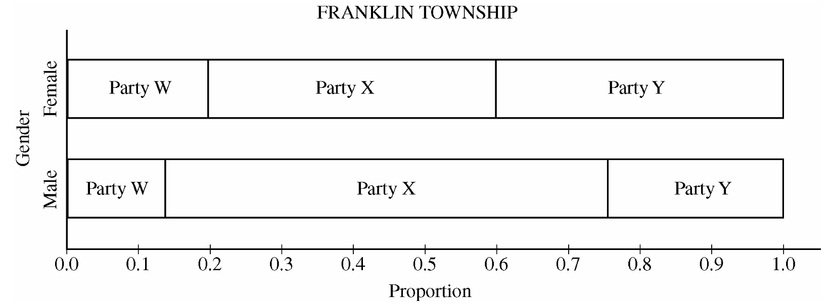
Most-appropriate topic codes (AP Statistics):
• Topic 2.7 — Independent Events and Unions of Events (Part b)
• Topic 2.1 — Tabular and Graphical Representations for the Distributions of Two Categorical Variables (Part c)
▶️ Answer/Explanation
(a)
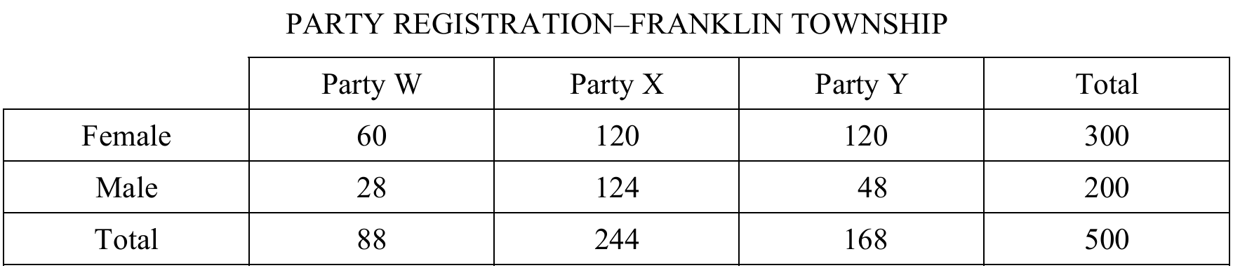
We need to find the conditional probability that a voter is registered for Party Y, given they are male. Looking only at the “Male” row, there are $200$ total males, and $48$ of them are registered for Party Y.
$P(\text{Party Y} \mid \text{Male}) = \frac{48}{200} = 0.24$
(b)
No, the events “is a male” and “is registered for Party Y” are not independent.
Two events $A$ and $B$ are independent if $P(A \mid B) = P(A)$. Let’s compare the conditional probability from part (a) to the overall marginal probability of being registered for Party Y.
$P(\text{Party Y}) = \frac{168}{500} = 0.336$
Since $P(\text{Party Y} \mid \text{Male}) = 0.24$ and $P(\text{Party Y}) = 0.336$, the probabilities are not equal ($0.24 \neq 0.336$). Knowing that a randomly selected voter is male changes the probability that they are registered for Party Y, so the events are dependent.
(c)
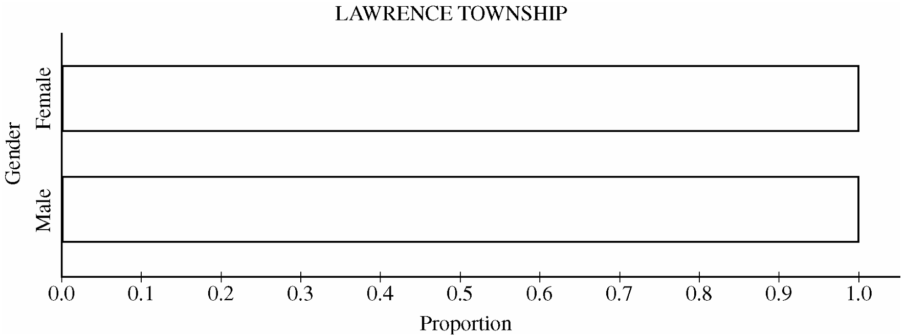
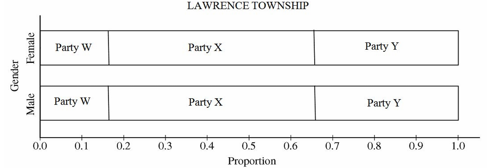
Because party registration is independent of gender in Lawrence Township, the distribution of party registration for both males and females must be identical to the overall marginal distribution of the town.
We first calculate the overall proportions for each party (which are the same as Franklin Township’s overall proportions):
Party W: $\frac{88}{500} = 0.176$
Party X: $\frac{244}{500} = 0.488$
Party Y: $\frac{168}{500} = 0.336$
To complete the segmented bar graph, you would draw identical bars for both the Male and Female categories with the following dividing lines:
• The segment for Party W starts at $0.0$ and ends at $0.176$.
• The segment for Party X starts at $0.176$ and ends at $0.176 + 0.488 = 0.664$.
• The segment for Party Y starts at $0.664$ and extends to $1.0$.
Question
Most-appropriate topic codes (AP Statistics):
• Topic 2.6 — Conditional Probability (Part b)
• Topic 2.7 — Independent Events and Unions of Events (Part c)
• Topic 3.4 — Justifying a Claim Based on a Confidence Interval for a Population Proportion (Part d)
▶️ Answer/Explanation
(a)
We want to construct a 99% confidence interval for the true proportion $p$.
First, calculate our point estimate and confirm design guidelines:
$\hat{p} = \frac{2,688}{9,600} = 0.28$
$n\hat{p} = 2,688 \ge 10 \quad \text{and} \quad n(1-\hat{p}) = 9,600 – 2,688 = 6,912 \ge 10$
The sample is random, and success/failure counts are well above 10, satisfying normality criteria. Using critical value $z^* = 2.576$:
$\text{Margin of Error} = z^* \sqrt{\frac{\hat{p}(1-\hat{p})}{9,600}} = 2.576 \sqrt{\frac{0.28 \times 0.72}{9,600}} = 2.576 \times 0.004583 = 0.0118$
$\text{Interval} = 0.28 \pm 0.0118 \rightarrow (0.2682, 0.2918)$
Interpretation: We are 99% confident that the true proportion of all United States twelfth-grade students who would answer this history question correctly is between $0.2682$ and $0.2918$.
(b)
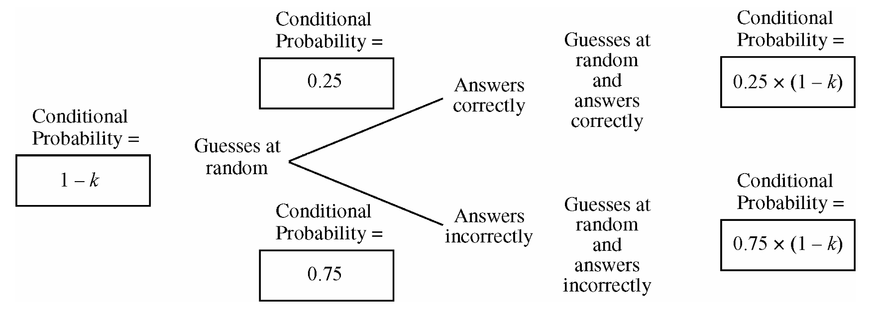
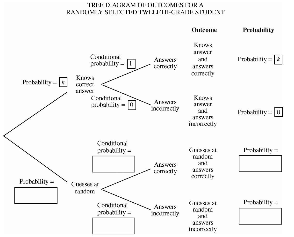
The branches are filled based on the structural logic given in the problem prompt:
• The top initial branch represents the probability a student Knows the answer, which is: $k$
• The bottom initial branch represents the probability a student Does not know the answer, which is: $1 – k$
• Given they know the answer, they choose the correct option with absolute certainty, making the conditional probability of a Correct response: $1$
• Given they do not know the answer, they choose by random guessing out of 4 options, making the conditional probability of a Correct response: $\frac{1}{4} = 0.25$
(c)
To find the overall proportion $p$ of correct answers, accumulate the final correct path terminals from your tree model:
$p = P(\text{Knows}) \times P(\text{Correct} \mid \text{Knows}) + P(\text{Doesn’t Know}) \times P(\text{Correct} \mid \text{Doesn’t Know})$
$p = k(1) + (1-k)(0.25)$
$p = k + 0.25 – 0.25k = 0.75k + 0.25$
(d)
To construct a 99% interval for $k$, isolate $k$ from our part (c) linear transformation model:
$p = 0.75k + 0.25 \implies p – 0.25 = 0.75k \implies k = \frac{p – 0.25}{0.75}$
Now, substitute the lower and upper bounds of $p$ from part (a) into this equation:
$\text{Lower Bound for } k = \frac{0.2682 – 0.25}{0.75} = \frac{0.0182}{0.75} = 0.0243$
$\text{Upper Bound for } k = \frac{0.2918 – 0.25}{0.75} = \frac{0.0418}{0.75} = 0.0557$
The resulting 99% confidence interval for the proportion of students who actually know the answer is $(0.0243, 0.0557)$.
Question
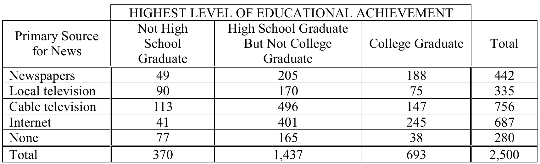
(d) The company wants to conduct a statistical test to investigate whether there is an association between educational achievement and primary source for news for adults in the city. What is the name of the statistical test that should be used?
Most-appropriate topic codes (AP Statistics):
• Topic \(2.6\) — Conditional Probability (Part \(\mathrm{b}\))
• Topic \(2.7\) — Independent Events and Unions of Events (Parts \(\mathrm{a}\), \(\mathrm{c}\))
• Topic \(3.14\) — Setting Up a Chi-Square Test for Homogeneity or Independence (Part \(\mathrm{d}\))
▶️ Answer/Explanation
(a)
Let \(C\) = event that the adult is a college graduate, and \(I\) = event that the adult obtains news primarily from the internet.
Using the Addition Rule:
\(P(C \cup I) = P(C) + P(I) – P(C \cap I)\)
Reading the values directly from the table:
\(P(C) = \frac{693}{2500}, \qquad P(I) = \frac{687}{2500}, \qquad P(C \cap I) = \frac{245}{2500}\)
\(P(C \cup I) = \frac{693}{2500} + \frac{687}{2500} – \frac{245}{2500} = \frac{693 + 687 – 245}{2500} = \frac{1135}{2500}\)
\(\boxed{P(C \cup I) = \frac{1135}{2500} = 0.454}\)
Don’t forget to subtract the overlap — college graduates who use the internet get counted in both the college graduate total and the internet total, so we subtract them once to avoid double-counting.
(b)
We want the conditional probability that an adult obtains news from the internet, given that the adult is a college graduate. From the table, among the 693 college graduates, 245 primarily use the internet:
\(P(I \mid C) = \frac{P(C \cap I)}{P(C)} = \frac{\dfrac{245}{2500}}{\dfrac{693}{2500}} = \frac{245}{693}\)
\(\boxed{P(I \mid C) = \frac{245}{693} \approx 0.354}\)
This is a conditional probability — we’ve already restricted our pool to only the 693 college graduates, so 693 becomes the new denominator. The 2,500 total cancels out entirely.
(c)
Two events are independent if and only if \(P(A \cap B) = P(A) \cdot P(B)\), which is equivalent to checking whether \(P(I \mid C) = P(I)\).
From the table:
\(P(I) = \frac{687}{2500} = 0.275\)
\(P(I \mid C) = \frac{245}{693} \approx 0.354\)
Since \(P(I \mid C) \approx 0.354 \neq 0.275 = P(I)\), the two events are not independent.
We can also verify using the multiplication rule directly:
\(P(C) \cdot P(I) = \frac{693}{2500} \times \frac{687}{2500} = \frac{476{,}091}{6{,}250{,}000} \approx 0.0762\)
\(P(C \cap I) = \frac{245}{2500} = 0.098\)
Since \(0.098 \neq 0.0762\), the events are confirmed to be not independent. In real terms, college graduates are noticeably more likely to get their news from the internet than the general adult population — that difference in rates is exactly what “not independent” means here.
(d)
The appropriate test is the Chi-Square Test of Association (or Independence).
This test is used when we want to determine whether there is an association between two categorical variables — here, educational achievement (3 categories) and primary news source (5 categories).
The degrees of freedom are calculated as:
\(\text{df} = (\text{number of rows} – 1) \times (\text{number of columns} – 1)\)
\(\text{df} = (5 – 1) \times (3 – 1) = 4 \times 2 = \boxed{8}\)
There are 5 rows (news source categories) and 3 columns (education levels), not counting the totals row and column. The degrees of freedom formula captures how many cells in the table are “free to vary” once the row and column totals are fixed.
Question
Most-appropriate topic codes (AP Statistics):
• Topic \(2.7\) — Independent Events and Unions of Events (Part \(\mathrm{c}\))
• Topic \(2.5\) — Mutually Exclusive Events (Part \(\mathrm{c}\), complement rule)
▶️ Answer/Explanation
(a)
Out of the 500 blood samples known to not contain HIV, the ELISA returned a positive result for 37 of them.
So the estimated probability that the ELISA is positive given no HIV is:
\(P(\text{positive} \mid \text{no HIV}) = \frac{37}{500} = 0.074\)
\(\boxed{P(\text{positive} \mid \text{no HIV}) \approx 0.074}\)
(b)
First, find the total number of blood samples that returned a positive ELISA result across both groups:
\(489 + 37 = 526 \text{ positive results in total}\)
Of those 526 positive results, 489 actually came from samples that truly contained HIV.
So the proportion of positive ELISA results that actually contained HIV is:
\(\frac{489}{526} \approx 0.9297\)
\(\boxed{\frac{489}{526} \approx 0.9297}\)
(c)
From part (a), the probability the ELISA is positive for a sample with no HIV is \(0.074\), and therefore the probability it is negative is \(1 – 0.074 = 0.926\).
A sample with no HIV will be sent for the expensive test if: the 1st ELISA is positive AND at least one of the 2 follow-up ELISAs is also positive.
Find the probability that at least one of the two follow-up tests is positive (using the complement):
\(P(\text{at least one positive in 2 follow-ups}) = 1 – P(\text{both negative}) = 1 – (0.926)^2\)
\(= 1 – 0.857476 = 0.142524\)
Now multiply by the probability the first ELISA is positive:
\(P(\text{subjected to expensive test}) = (0.074)(0.142524)\)
\(= 0.010547\)
\(\boxed{P(\text{subjected to expensive test}) \approx 0.0105}\)
Question
Most-appropriate topic codes (AP Statistics):
• Topic 2.6 — Conditional Probability (Part b)
• Topic 2.7 — Independent Events and Unions of Events (Part c)
• Topic 2.2 — Summary Statistics for Two Categorical Variables (Part a)
▶️ Answer/Explanation
(a)
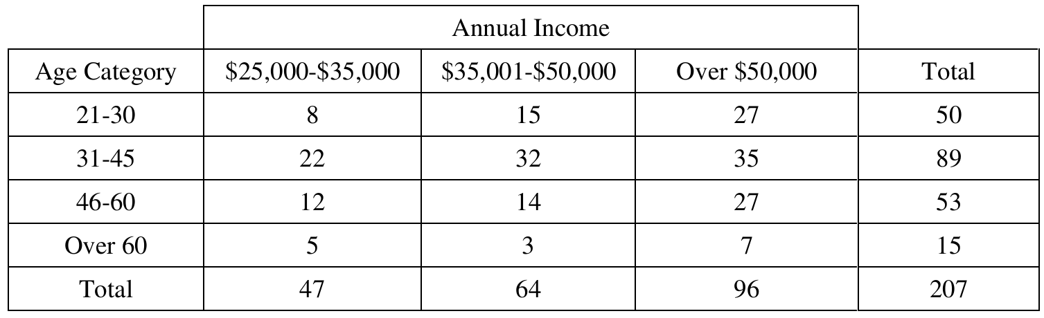
We want the probability that a randomly selected person from the sample falls in the 31–45 age category.
The total number of people in the sample is 207, and the number in the 31–45 age group is 89.
\( P(\text{age } 31\text{–}45) = \frac{89}{207} \approx 0.42995 \)
\(\boxed{P(\text{age } 31\text{–}45) \approx 0.4300}\)
(b)
We now want the conditional probability that a person is in the 31–45 age category, given that their income is over \(\$50{,}000\).
From the table, the total number of people with income over \(\$50{,}000\) is 96, and among those, 35 are in the 31–45 age group.
\( P(\text{age } 31\text{–}45 \mid \text{income over } \$50{,}000) = \frac{35}{96} \approx 0.36458 \)
\(\boxed{P(\text{age } 31\text{–}45 \mid \text{income over } \$50{,}000) \approx 0.3646}\)
(c)
For two variables to be independent, knowing the value of one variable should not change the probability of the other — in other words, the marginal probability and the conditional probability must be equal.
From part (a), \(P(\text{age } 31\text{–}45) \approx 0.4300\), and from part (b), \(P(\text{age } 31\text{–}45 \mid \text{income over } \$50{,}000) \approx 0.3646\).
Since these two probabilities are not equal (\(0.4300 \neq 0.3646\)), knowing a person’s income category does change the probability of being in the 31–45 age group.
Therefore, annual income and age category are not independent for those in this sample.