
AP Statistics 2.8 Introduction to Random Variables and Probability Distributions- Exam Style Questions - FRQs - New Syllabus
Question
ii. Calculate the standard deviation of the distribution of the number of geodes Sarah will open until a red crystal is found. Show your work.

ii. Calculate \(P(Y=4)\). Show your work.
ii. Interpret the mean of the distribution of the number of geodes Conrad will open, which was calculated in part (c-i).
Most-appropriate topic codes (AP Statistics):
• Topic \(2.9\) — Parameters of Random Variables (Parts \( \mathrm{a} \), \( \mathrm{c} \))
▶️ Answer/Explanation
(a)
i. Since Sarah opens geodes until she finds a red crystal, the number of geodes she opens follows a geometric distribution with a probability of success \(p = 0.08\).
The mean (expected value) of a geometric distribution is \(\mu = \dfrac{1}{p}\).
\(\mu = \dfrac{1}{0.08} = 12.5\) geodes.
ii. The standard deviation of a geometric distribution is given by \(\sigma = \dfrac{\sqrt{1-p}}{p}\).
\(\sigma = \dfrac{\sqrt{1-0.08}}{0.08} = \dfrac{\sqrt{0.92}}{0.08} \approx 11.99\) geodes.
(b)
i. The probability that Conrad opens exactly \(3\) geodes is the probability of finding non-red crystals in the first two attempts and a red crystal on the third attempt.
\(P(Y=3) = (1 – 0.08)^2(0.08) = (0.92)^2(0.08) \approx 0.067712\).
ii. The probability that Conrad opens \(4\) geodes is the probability that he does not stop in the first \(3\) geodes. He will open 4 geodes whether the 4th is red or not.
\(P(Y=4) = 1 – P(Y \le 3)\)
\(P(Y=4) = 1 – (0.08 + 0.0736 + 0.067712) \approx 0.778688\).
(c)
i. The mean of the discrete probability distribution for \(Y\) is the expected value, calculated by summing the products of each outcome and its respective probability.
\(\mu_Y = E(Y) = 1(0.08) + 2(0.0736) + 3(0.067712) + 4(0.778688)\)
\(\mu_Y \approx 0.08 + 0.1472 + 0.203136 + 3.114752 \approx 3.545\) geodes.
ii. The mean of \(3.545\) represents the average number of geodes Conrad would open per game if he were to play this game many, many times under the exact same stopping rules.
Question

(ii) Calculate the proportion of bath fizzies that contain at least $\$10$.
Most-appropriate topic codes (AP Statistics):
• Topic \(2.8\) — Introduction to Random Variables and Probability Distributions (Part \( \mathrm{a} \))
• Topic \(2.9\) — Parameters of Random Variables (Parts \( \mathrm{c} \), \( \mathrm{d} \))
▶️ Answer/Explanation
(a) (i)
$P(X = 1) = 1 – (0.2 + 0.05 + 0.05 + 0.01 + 0.01)$
$P(X = 1) = 1 – 0.32$
$P(X = 1) = 0.68$
(a) (ii)
$P(X \ge 10) = P(X = 10) + P(X = 20) + P(X = 50) + P(X = 100)$
$P(X \ge 10) = 0.05 + 0.05 + 0.01 + 0.01$
$P(X \ge 10) = 0.12$
(b)
$P(X = 100 \mid X \ge 10) = \frac{P(X = 100 \text{ and } X \ge 10)}{P(X \ge 10)}$
$P(X = 100 \mid X \ge 10) = \frac{0.01}{0.12}$
$P(X = 100 \mid X \ge 10) \approx 0.0833 \text { or } \frac{1}{12} $
(c)
$E(X) = \sum [x \cdot P(x)]$
$E(X) = 1(0.68) + 5(0.2) + 10(0.05) + 20(0.05) + 50(0.01) + 100(0.01)$
$E(X) = 0.68 + 1 + 0.5 + 1 + 0.5 + 1$
$E(X) = \$4.68$
Interpretation: If many, many bath fizzies are randomly selected, the long-run average cash prize per fizzy will be approximately $\$4.68$.
(d)
$E(\text{euros}) = 0.89 \times E(X)$
$E(\text{euros}) = 0.89 \times 4.68$
$E(\text{euros}) \approx 4.1652 \text{ euros}$
Question
Most-appropriate topic codes (AP Statistics):
• Topic \(2.9\) — Parameters of Random Variables (Part \( \mathrm{c} \))
• Topic \(2.11\) — The Normal Distribution (Parts \( \mathrm{a} \), \( \mathrm{b} \))
▶️ Answer/Explanation
(a)
We need to find the \(25\text{th}\) percentile of the normal distribution.
Looking at the standard normal distribution table, the \(z\)-score that corresponds to a left-tail area of \(0.25\) is approximately \(-0.6745\).
We can set up the formula for the \(z\)-score and solve for \(x\):
\(z = \dfrac{x – \mu}{\sigma}\)
\(-0.6745 = \dfrac{x – 30}{8}\)
\(x = 30 + 8(-0.6745) \approx 24.6\)
It is expected that \(25\) percent of the batteries will no longer work after approximately \(24.6\) months.
(b)
We are looking for the probability that the battery lifespan is less than \(24\) months.
First, we calculate the \(z\)-score for \(x = 24\):
\(z = \dfrac{24 – 30}{8}\)
\(z = -0.75\)
Using the standard normal probability table, the probability \(P(Z < -0.75)\) is roughly \(0.2266\).
The probability that the customer will require a replacement is \(0.2266\).
(c)
Let \(X\) represent the company’s financial gain per warranty purchased.
The probability that a replacement is required is \(0.2266\), resulting in a loss of \(\$150\).
The probability that a replacement is NOT required is \(1 – 0.2266 = 0.7734\), resulting in a gain of \(\$50\).
The expected value \(E(X)\) is the sum of each outcome multiplied by its corresponding probability:
\(E(X) = (50)(0.7734) + (-150)(0.2266)\)
\(E(X) = 38.67 – 33.99\)
\(E(X) = \$4.68\)
The expected gain for the company per warranty purchased is \(\$4.68\).
Question
If heads, you must respond no, regardless of whether you regularly recycle. If tails, please truthfully respond yes or no.
Most-appropriate topic codes (AP Statistics):
• Topic \(2.6\) — Conditional Probability (Part \( \mathrm{c}\text{-}\mathrm{ii} \))
• Topic \(2.8\) — Introduction to Random Variables and Probability Distributions (Part \( \mathrm{c}\text{-}\mathrm{i} \))
• Topic \(3.3\) — Constructing a Confidence Interval for a Population Proportion (Part \( \mathrm{a} \))
▶️ Answer/Explanation
(a)
The sample selected by the environmental science teacher contained $60$ students.
Detailed Solution:
First, find the point estimate $\hat{p}$ which is the midpoint of the confidence interval: $\hat{p} = \frac{0.584 + 0.816}{2} = 0.70$.
Next, determine the margin of error ($ME$) by calculating the distance from the midpoint to an endpoint: $ME = 0.816 – 0.70 = 0.116$.
Using the margin of error formula $ME = z^* \sqrt{\frac{\hat{p}(1-\hat{p})}{n}}$ for a $95\%$ confidence level ($z^* = 1.96$), we set up the equation $0.116 = 1.96 \sqrt{\frac{0.70(1-0.70)}{n}}$.
Solving for $n$ gives us $\sqrt{n} = \frac{1.96 \sqrt{0.21}}{0.116} \approx 7.74$, which squares to $n \approx 59.9$, revealing that the teacher’s sample size is exactly $60$ students.
(b)
Bias might have been introduced because students were asked directly by their environmental science teacher, which likely creates response bias.
Detailed Solution:
Because the survey is conducted face-to-face by a teacher who is expected to care about the environment, students may feel strong social pressure to give the “desirable” answer.
This phenomenon is known as response bias, where respondents do not answer truthfully in order to avoid judgment or please the interviewer.
As a result, more students will claim they recycle than actually do, artificially inflating the number of “yes” responses and causing the point estimate to be higher than the true population proportion.
(c)(i)
The expected number of students required to respond “no” due to the coin flip is $150$.
Detailed Solution:
Since the students are flipping a fair coin, the theoretical probability of getting heads is exactly $0.5$.
With a total random sample of $n = 300$ students, the expected number of heads is calculated as $n \times p = 300 \times 0.5$.
Therefore, we can expect exactly half the students, or $150$, to be forced to respond “no” based on the coin flip instructions.
(c)(ii)
The point estimate for the proportion of all students at the high school who would respond “yes” is $0.58$.
Detailed Solution:
Out of the $300$ total students, $213$ responded “no”, and we expect $150$ of these “no” responses to come from the students who flipped heads.
This means the remaining $213 – 150 = 63$ “no” responses came from the $150$ students who flipped tails and answered truthfully about not recycling.
Since $150$ students flipped tails and $63$ of them truthfully said “no”, the remaining $150 – 63 = 87$ students must have truthfully answered “yes”.
Thus, the point estimate for the proportion of students who actually recycle is $\frac{87}{150} = 0.58$.
Question

Most-appropriate topic codes (AP Statistics):
• Topic \(2.8\) — Introduction to Random Variables and Probability Distributions (Part \( \mathrm{a} \))
• Topic \(2.9\) — Parameters of Random Variables (Parts \( \mathrm{b} \), \( \mathrm{d} \))
▶️ Answer/Explanation
(a)
The probability that at least one ATM is working when the mall opens is the sum of the probabilities for \(1\), \(2\), and \(3\) ATMs.
\( P(X \ge 1) = 0.21 + 0.40 + 0.24 \)
\( P(X \ge 1) = 0.85 \)
(b)
The expected value of the number of ATMs that are working when the mall opens is found by multiplying each possible value by its corresponding probability and summing the results.
\( E(X) = 0(0.15) + 1(0.21) + 2(0.40) + 3(0.24) \)
\( E(X) = 0 + 0.21 + 0.80 + 0.72 \)
\( E(X) = 1.73 \text{ machines} \)
(c)
The probability that all three ATMs are working given that at least one ATM is working is calculated using the conditional probability formula.
\( P(X=3 \mid X \ge 1) = \dfrac{P(X=3 \text{ and } X \ge 1)}{P(X \ge 1)} \)
\( P(X=3 \mid X \ge 1) = \dfrac{P(X=3)}{P(X \ge 1)} \)
\( P(X=3 \mid X \ge 1) = \dfrac{0.24}{0.85} \approx 0.282 \)
(d)
Given that at least one ATM is working, the expected value would be greater than the expected value calculated in part (b).
By eliminating the possibility of \(0\) working ATMs, the probabilities for \(1\), \(2\), and \(3\) working ATMs all increase proportionally because they must now sum to \(1\). Since the higher values of \(X\) now have a higher probability of occurring relative to the total, the overall expected value must increase.
Question
Most-appropriate topic codes (AP Statistics):
• Topic \(2.8\) — Simulation and Random Variables (Part \( \mathrm{c} \))
▶️ Answer/Explanation
(a)
We use the multiplication rule for dependent events (sampling without replacement). At each step, the number of women and total people remaining both decrease:
\(P(\text{1st is a woman}) = \dfrac{3}{9}\)
\(P(\text{2nd is a woman} \mid \text{1st is a woman}) = \dfrac{2}{8}\)
\(P(\text{3rd is a woman} \mid \text{first two are women}) = \dfrac{1}{7}\)
Multiplying these together:
\(P(\text{all three are women}) = \dfrac{3}{9} \times \dfrac{2}{8} \times \dfrac{1}{7} = \dfrac{6}{504} = \dfrac{1}{84} \approx 0.012\)
\(\boxed{P(\text{all three are women}) \approx 0.012}\)
(b)
Yes, there is reason to doubt the manager’s claim. The probability calculated in part (a) shows that if the selection truly were random, there would only be about a \(1.2\%\) chance of all three selected people being women. Because this probability is so small, it is unlikely that this outcome would occur by chance alone, which gives us reasonable grounds to question whether the selection was truly made at random.
(c)
No, the proposed simulation does not correctly simulate the random selection of 3 women from the group of 9 people. Here is why:
In the actual selection, people are chosen without replacement — once a person is selected, they cannot be chosen again, so the probability of selecting a woman changes after each pick:
\(P(\text{woman on 1st pick}) = \dfrac{3}{9}, \quad P(\text{woman on 2nd pick} \mid \text{1st was a woman}) = \dfrac{2}{8}, \quad \ldots\)
In the dice simulation, however, the three dice rolls are independent of one another — the outcome of one die has no effect on the others. This effectively simulates sampling with replacement, where the probability of selecting a woman remains a fixed \(\dfrac{1}{3}\) on every roll.
Because the simulation uses independent dice rolls rather than dependent draws without replacement, it does not correctly model the actual random selection process.
Question

Most-appropriate topic codes (AP Statistics):
• Topic 2.9 — Parameters of Random Variables (Parts b, c)
• Topic 2.12 — Sampling Distributions and the Central Limit Theorem (Part d)
▶️ Answer/Explanation
(a)
The random variable \(X\) is defined as the net contribution to the charity, which is equal to: \(\text{Donation Received} – \text{Payout Amount}\).
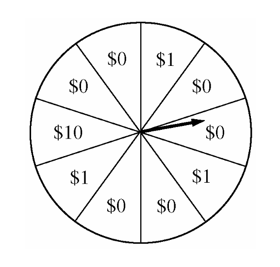
• For a payout of \$0, the net contribution is: \(\$2 – \$0 = \$2\). There are 6 sectors labeled \$0 out of 10 total sectors.
• For a payout of \$1, the net contribution is: \(\$2 – \$1 = \$1\). There are 3 sectors labeled \$1 out of 10 total sectors.
• For a payout of \$10, the net contribution is: \(\$2 – \$10 = -\$8\). There is 1 sector labeled \$10 out of 10 total sectors.
The completed probability distribution table is:

(b)
The expected value of the net contribution for a single play is calculated using the formula: \(E(X) = \sum x_i P(x_i)\).
\(E(X) = (\$2)(0.6) + (\$1)(0.3) + (-\$8)(0.1)\)
\(E(X) = 1.2 + 0.3 – 0.8\)
\(E(X) = \$0.70\)
The expected net contribution to the charity per play is \(\$0.70\).
(c)
Let \(n\) be the number of times the game is played.
The total expected net contribution for \(n\) plays is: \(E(\text{Total}) = n \cdot E(X) = 0.70n\).
We want the total expected net contribution to be at least \$500:
\(0.70n \ge 500\)
\(n \ge \dfrac{500}{0.70}\)
\(n \ge 714.29\)
Since the number of plays must be an integer, the game must be played a minimum of \(715\) times.
(d)
Let \(W\) represent the total net contribution from 1,000 plays of the game.
We are given that \(W\) is approximately normally distributed with a mean of \(\mu_W = \$700\) and a standard deviation of \(\sigma_W = \$92.79\).
We want to find the probability that the net contribution is at least \$500: \(P(W \ge 500)\).
First, compute the standardized \(z\)-score:
\(z = \dfrac{500 – \mu_W}{\sigma_W} = \dfrac{500 – 700}{92.79} = \dfrac{-200}{92.79} \approx -2.16\)
Using the standard normal probability table, the probability lying below \(z = -2.16\) is \(0.0154\).
Therefore, the probability of obtaining a net contribution of at least \$500 is:
\(P(Z \ge -2.16) = 1 – 0.0154 = 0.9846\).
The normal approximation for the probability is approximately \(0.9846\).
Question

Most-appropriate topic codes (AP Statistics):
• Topic 2.10 — The Binomial Distribution (Parts a, b)
• Topic 1.11 — Random Sampling (Part c)
▶️ Answer/Explanation
(a)
Because the total population ($297,354$) is overwhelmingly large compared to the sample size ($2,000$), we can treat this as a binomial distribution even though sampling is without replacement.
The probability of selecting a model E owner is $p = \dfrac{2,323}{297,354} \approx 0.007812$.
The sample size is $n = 2000$.
Expected number (Mean):
$\mu_E = n \times p = 2000 \times 0.007812 \approx 15.62$ owners
Standard Deviation:
$\sigma_E = \sqrt{n \times p \times (1-p)} = \sqrt{2000 \times 0.007812 \times (1 – 0.007812)} = \sqrt{15.49} \approx 3.93$ owners
(b)
For the reason given in part (a), the binomial distribution with $n = 2,000$ and $p \approx 0.0078$ can be used here. The probability that the sample would contain fewer than 12 owners of model E is calculated from the binomial distribution to be $\sum_{x=0}^{11} \binom{2,000}{x} (0.0078)^x (0.9922)^{2,000-x} \approx 0.147$. This probability is small enough that the result (fewer than 12 owners of model E in the sample) is not likely, but this probability is also not small enough to consider the result very unlikely.
This binomial probability can also be evaluated using a normal approximation. This is reasonable because $n \times p = (2,000) \times (0.0078) = 15.6$ is larger than 10 and $n(1 – p) = (2,000) \times (0.9922) = 1,984.4$ is much larger than 10. Using the mean and standard deviation from part (a) gives
$P(X \le 11) \approx P\left( Z < \dfrac{12.0 – 15.62}{3.94} \right) = P(Z < -0.92) = 0.179$.
(c)
To guarantee at least 12 owners from each model, the company should use a stratified random sampling method.
The researcher should use the five car models as the strata.
They can determine how many individuals they want to sample from each model (stratum) as long as every model’s assigned sample size is $12$ or greater, and all five sizes add up to exactly $2,000$.
Then, they simply perform five separate simple random samples—one within each specific car model’s list of owners—to achieve the decided quota for that model.
Question
\(H_a\): There is a difference in the distributions of hurricane damage amounts among the three regions.
Most-appropriate topic codes (AP Statistics):
• Topic 2.8 — Introduction to Random Variables and Probability Distributions (Part c)
• Topic 3.15 — Carrying Out a Chi-Square Test for Homogeneity or Independence (Parts d, e)
▶️ Answer/Explanation
(a) Graphical Display
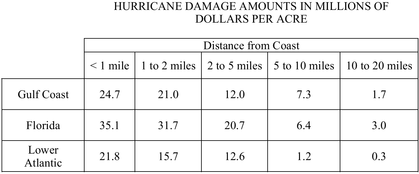
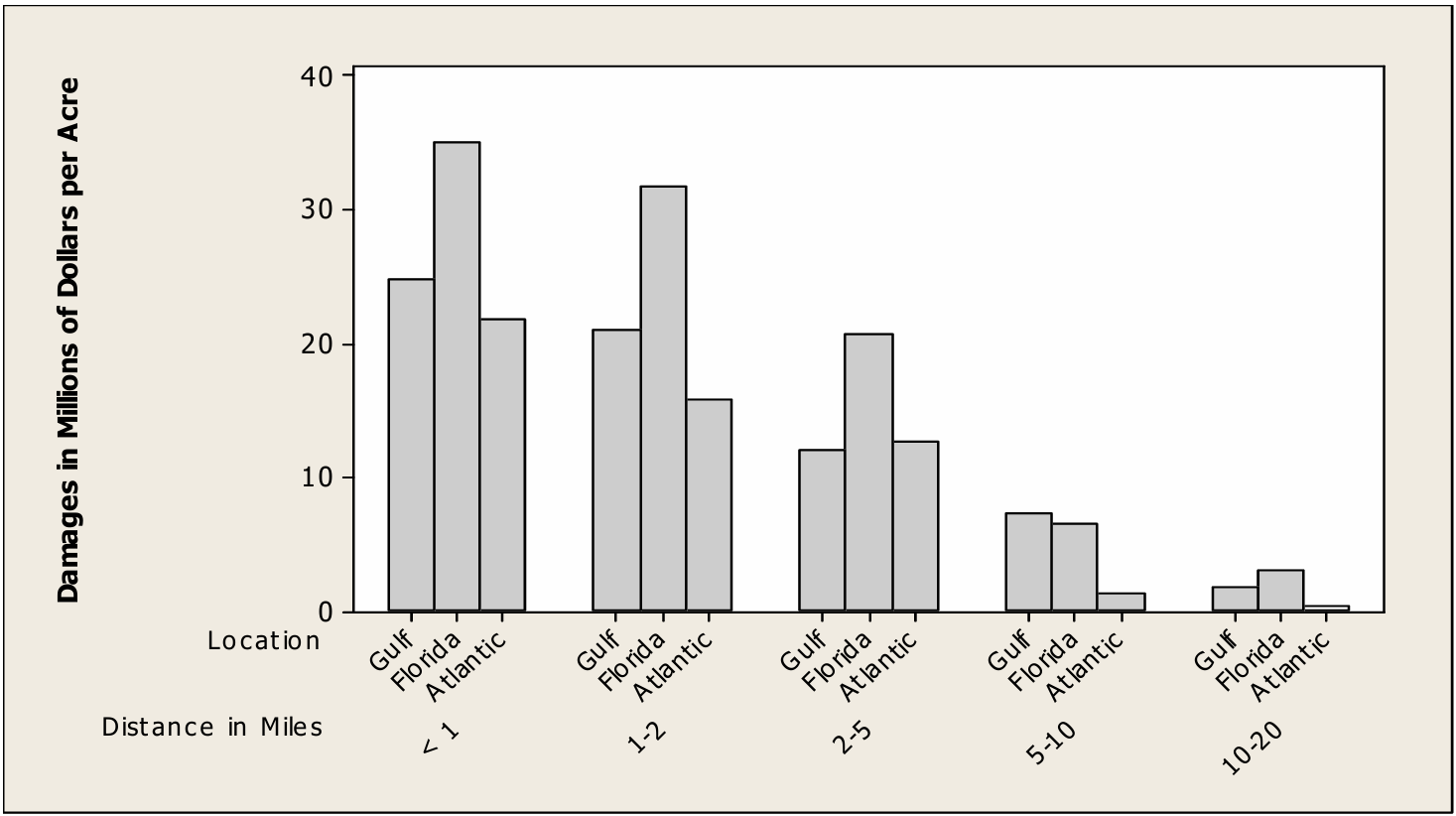
A well-constructed graphical display for this data is a grouped bar chart, with the five distance-from-coast categories on the horizontal axis and damage amounts (in millions of dollars per acre) on the vertical axis. Three bars are drawn side by side within each distance group — one for Gulf Coast, one for Florida, and one for Lower Atlantic — with a clearly labeled key.
(b) Differences and Similarities
Similarity: In all three regions, hurricane damage amounts decrease consistently as distance from the coast increases. This pattern holds without exception across all five distance categories for every region.
Difference: For almost every distance category, Florida has the highest damage amounts, while the Lower Atlantic region generally has the lowest. The Gulf Coast falls in between, though at the 5-to-10-mile distance, the Gulf Coast actually has the highest damage of the three regions.
(c) Missing Ranks and Average Ranks
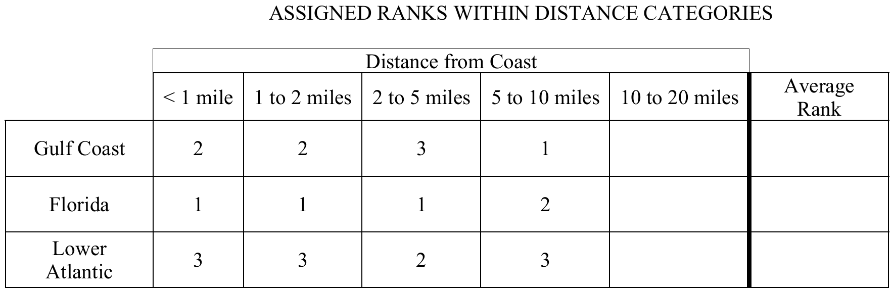
For the 10-to-20-miles distance category, compare the three damage amounts:
Florida: \(3.0\) million (highest) \(\Rightarrow\) rank \(= 1\)
Gulf Coast: \(1.7\) million (middle) \(\Rightarrow\) rank \(= 2\)
Lower Atlantic: \(0.3\) million (lowest) \(\Rightarrow\) rank \(= 3\)
The completed rank table is:

The average ranks are computed as follows:
\(\bar{R}_G = \frac{2+2+3+1+2}{5} = \frac{10}{5} = 2.0\)
\(\bar{R}_F = \frac{1+1+1+2+1}{5} = \frac{6}{5} = 1.2\)
\(\bar{R}_A = \frac{3+3+2+3+3}{5} = \frac{14}{5} = 2.8\)
(d) Calculating the Test Statistic \(Q\)
Substitute the average ranks from part (c) into the formula:
\(Q = 5\left[\left(\bar{R}_G – 2\right)^2 + \left(\bar{R}_F – 2\right)^2 + \left(\bar{R}_A – 2\right)^2\right]\)
\(Q = 5\left[(2.0 – 2)^2 + (1.2 – 2)^2 + (2.8 – 2)^2\right]\)
\(Q = 5\left[0 + (-0.8)^2 + (0.8)^2\right]\)
\(Q = 5\left[0 + 0.64 + 0.64\right]\)
\(\boxed{Q = 5 \times 1.28 = 6.4}\)
(e) Simulation-Based Conclusion
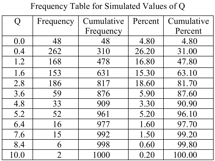
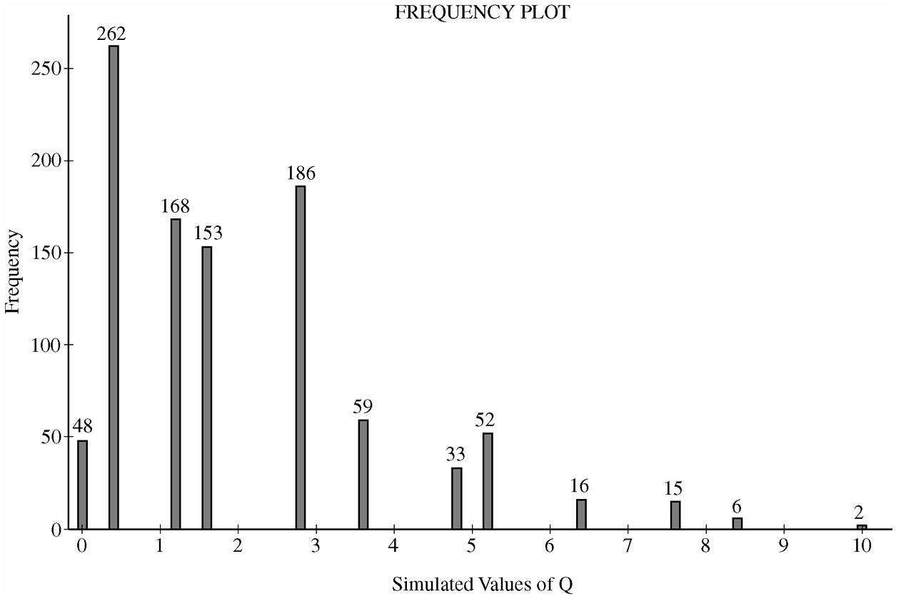
From the frequency table, simulated \(Q\) values of \(6.4\) or greater occurred in:
\(16 + 15 + 6 + 2 = 39 \text{ out of } 1{,}000 \text{ simulations}\)
This gives an approximate \(p\)-value of:
\(p\text{-value} \approx \frac{39}{1{,}000} = 0.039\)
Since the \(p\)-value of \(0.039\) is less than \(\alpha = 0.05\), we reject \(H_0\). The sample data provide reasonably strong evidence that there is a difference in the distributions of hurricane damage amounts among the three coastal regions (Gulf Coast, Florida, and Lower Atlantic).
Question

Most-appropriate topic codes (AP Statistics):
• Topic \(2.9\) — Parameters of Random Variables (Part \(\mathrm{a}\))
• Topic \(2.7\) — Independent Events and Unions of Events (Parts \(\mathrm{b}\), \(\mathrm{c}\), \(\mathrm{d}\))
▶️ Answer/Explanation
(a)
The expected value (mean) of a discrete random variable is \(\mu = \sum x_i \cdot P(x_i)\). We apply this to each player’s distribution.
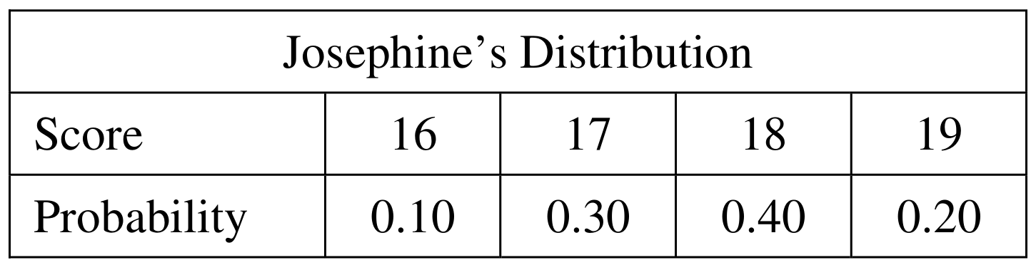
For Josephine:
\(\mu_J = 16(0.10) + 17(0.30) + 18(0.40) + 19(0.20)\)
\(\mu_J = 1.6 + 5.1 + 7.2 + 3.8 = \boxed{17.7}\)
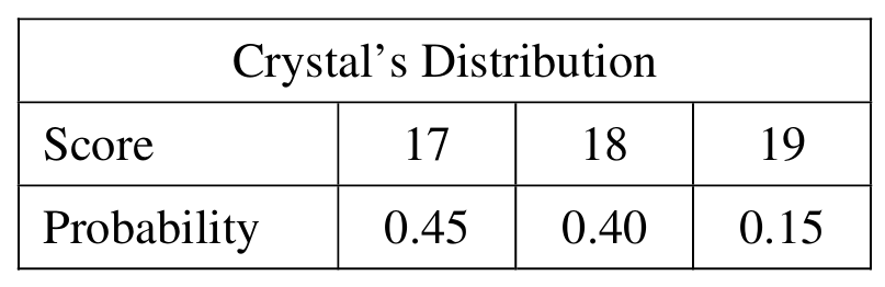
For Crystal:
\(\mu_C = 17(0.45) + 18(0.40) + 19(0.15)\)
\(\mu_C = 7.65 + 7.20 + 2.85 = \boxed{17.7}\)
Both players have the same expected score of \(17.7\).
(b)
We need all pairs \((J, C)\) such that \(J – C = -1\), i.e., Josephine’s score is exactly 1 less than Crystal’s. Since scores are independent, the probability of each pair is the product of the individual probabilities.
\(J = 16,\ C = 17\): \(\quad P = (0.10)(0.45) = 0.045\)
\(J = 17,\ C = 18\): \(\quad P = (0.30)(0.40) = 0.120\)
\(J = 18,\ C = 19\): \(\quad P = (0.40)(0.15) = 0.060\)
These are the only three combinations that produce a difference of \(-1\).
(c)
Since the three combinations in part (b) are mutually exclusive, we simply add their probabilities:
\(P(J – C = -1) = 0.045 + 0.120 + 0.060\)
\(\boxed{P(J – C = -1) = 0.225}\)
(d)
First, we find the missing probability for a difference of \(-2\). Since all probabilities in the distribution must sum to 1:
\(P(J – C = -2) = 1 – 0.015 – 0.225 – 0.325 – 0.260 – 0.090\)
\(P(J – C = -2) = 1 – 0.915 = \boxed{0.085}\)
The completed distribution table is:

Crystal’s score is higher than Josephine’s when the difference \(J – C < 0\), i.e., when the difference is \(-3\), \(-2\), or \(-1\).
\(P(\text{Crystal} > \text{Josephine}) = P(J – C < 0) = 0.015 + 0.085 + 0.225\)
\(\boxed{P(\text{Crystal} > \text{Josephine}) = 0.325}\)
Question
Most-appropriate topic codes (AP Statistics):
• Topic 2.9 — Parameters of Random Variables (Part \(\mathrm{a}\))
• Topic 2.11 — The Normal Distribution (Parts \(\mathrm{b}\), \(\mathrm{c}\))
▶️ Answer/Explanation
(a)
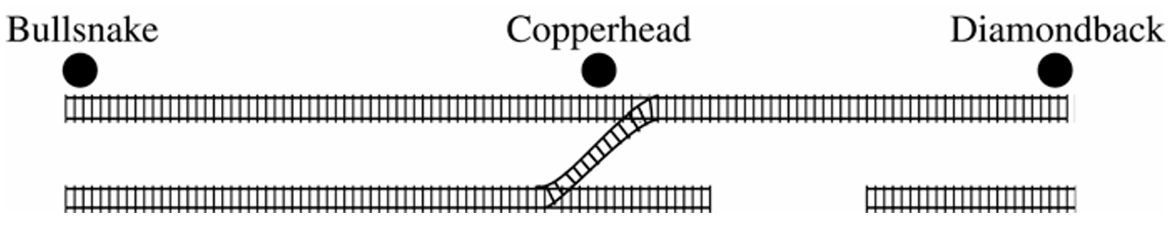
Since \(X\) and \(Y\) are independent normal random variables, their difference \(Y – X\) is also normally distributed. The mean and standard deviation of \(Y – X\) are found as follows:
\(\mu_{Y-X} = \mu_Y – \mu_X = 200 – 170 = 30 \text{ minutes}\)
\(\sigma_{Y-X} = \sqrt{\sigma_Y^2 + \sigma_X^2} = \sqrt{10^2 + 20^2} = \sqrt{100 + 400} = \sqrt{500} \approx 22.36 \text{ minutes}\)
\(\boxed{Y – X \sim N(30,\ 22.36^2)}\)
The distribution of \(Y – X\) is normal with mean \(30\) minutes and standard deviation \(22.36\) minutes (variance \(500\)).
(b)
The train from Bullsnake has to wait when it arrives at Copperhead before the train from Diamondback — that is, when \(X < Y\), or equivalently when \(Y – X > 0\).
Standardize to find the \(z\)-score:
\(z = \dfrac{0 – 30}{22.36} = \dfrac{-30}{22.36} \approx -1.34\)
So the required probability is:
\(P(Y – X > 0) = P\!\left(z > -1.34\right) = 1 – P(z < -1.34) = 1 – 0.0901 = 0.9099\)
\(\boxed{P(\text{wait}) \approx 0.91}\)
About \(91\%\) of days the train from Bullsnake will have to wait at Copperhead.
(c)
Let \(D\) be the delay (in minutes) added to the Bullsnake train’s departure. The new travel-plus-delay time for the Bullsnake train is \(X + D\), where \(D\) is a constant. The difference \(Y – (X + D)\) is then normally distributed with:
\(\mu_{Y-(X+D)} = 200 – (170 + D) = 30 – D\)
\(\sigma_{Y-(X+D)} = 22.36 \text{ (unchanged, since } D \text{ is constant)}\)
We want \(P\!\left(Y – (X+D) > 0\right) = 0.01\). This means the right-tail area above \(0\) equals \(0.01\), so the left-tail area below \(0\) equals \(0.99\). The corresponding \(z\)-score for \(0.99\) is \(z = 2.33\).
Setting up the equation:
\(z = \dfrac{0 – (30 – D)}{22.36} = 2.33\)
\(0 – (30 – D) = 2.33 \times 22.36\)
\(D – 30 = 52.10\)
\(D = 82.10 \text{ minutes}\)
\(\boxed{D \approx 82 \text{ minutes}}\)
The Snake Gulch Railroad should delay the departure of the train from Bullsnake by approximately \(82\) minutes so that the probability of having to wait drops to only \(0.01\).
Question
Most-appropriate topic codes (AP Statistics):
• Topic 2.10 — The Binomial Distribution (Part \(\mathrm{b}\))
• Topic 2.8 — Introduction to Random Variables and Probability Distributions (Parts \(\mathrm{a}\), \(\mathrm{b}\))
• Topic 2.12 — Sampling Distributions and the Central Limit Theorem (Part \(\mathrm{c}\))
• Topic 4.1 — Sampling Distributions for Sample Means (Part \(\mathrm{c}\))
▶️ Answer/Explanation
(a)
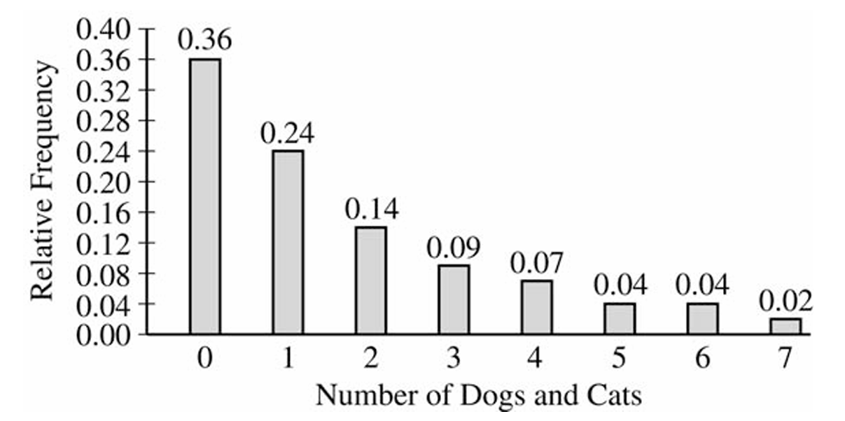
A household is in violation if it owns more than \(3\) pets, i.e., \(X > 3\). Read the relative frequencies for \(X = 4, 5, 6, 7\) directly from the graph and add them up.
\(P(X > 3) = P(X=4) + P(X=5) + P(X=6) + P(X=7)\)
\(P(X > 3) = 0.07 + 0.04 + 0.04 + 0.02\)
\(\boxed{P(X > 3) = 0.17}\)
(b)
Let \(Y\) = the number of households in violation among the \(10\) selected. Since each household is independently either in violation or not, \(Y\) follows a binomial distribution with \(n = 10\) and \(p = 0.17\) (from part (a)).
Using the binomial probability formula \(P(Y = k) = \dbinom{n}{k} p^k (1-p)^{n-k}\):
\(P(Y = 2) = \binom{10}{2}(0.17)^2(0.83)^8\)
\(P(Y = 2) = 45 \times (0.0289) \times (0.2252)\)
\(\boxed{P(Y = 2) \approx 0.2929}\)
(c)
Because the sample size \(n = 150\) is large, the Central Limit Theorem tells us the sampling distribution of \(\bar{X}\) will be approximately normal, regardless of the shape of the original population distribution.
The mean of the sampling distribution equals the population mean:
\(\mu_{\bar{X}} = \mu = 1.65\)
The standard deviation (standard error) of the sampling distribution is:
\(\sigma_{\bar{X}} = \dfrac{\sigma}{\sqrt{n}} = \dfrac{1.851}{\sqrt{150}} \approx 0.1511\)
So the sampling distribution of \(\bar{X}\) is approximately \(N(1.65,\ 0.1511)\) — normal, centered at \(1.65\), with a standard deviation of about \(0.1511\).
Question
Most-appropriate topic codes (AP Statistics):
• Topic 2.9 — Parameters of Random Variables (Parts a, b, c)
▶️ Answer/Explanation
(a)
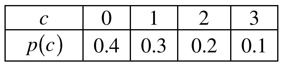
The mean of a discrete random variable is computed by multiplying each value by its probability and summing:
\( \mu_C = \sum c \cdot p(c) = (0)(0.4) + (1)(0.3) + (2)(0.2) + (3)(0.1) \)
\( \mu_C = 0 + 0.3 + 0.4 + 0.3 = \boxed{1} \)
For the standard deviation, first compute the variance using \(\sigma_C^2 = \sum (c – \mu_C)^2 \cdot p(c)\):
\( \sigma_C^2 = (0-1)^2(0.4) + (1-1)^2(0.3) + (2-1)^2(0.2) + (3-1)^2(0.1) \)
\( \sigma_C^2 = (1)(0.4) + (0)(0.3) + (1)(0.2) + (4)(0.1) = 0.4 + 0 + 0.2 + 0.4 = 1 \)
Taking the square root gives the standard deviation:
\( \boxed{\sigma_C = \sqrt{1} = 1} \)
It’s a neat coincidence here that the variance and standard deviation are both equal to 1 — don’t mix them up!
(b)
Let \(T = C + A\), where \(A\) is the number of adult tickets purchased. We are given \(\mu_A = 2\) and \(\sigma_A = 1.2\).
Since means always add regardless of independence:
\( \mu_T = \mu_C + \mu_A = 1 + 2 = \boxed{3} \)
Because \(C\) and \(A\) are independent, variances add (not standard deviations):
\( \sigma_T^2 = \sigma_C^2 + \sigma_A^2 = (1)^2 + (1.2)^2 = 1 + 1.44 = 2.44 \)
\( \sigma_T = \sqrt{2.44} \approx \boxed{1.562} \)
Remember: you can only add variances directly when the variables are independent — never add the standard deviations themselves.
(c)
Let \(M = 15C + 25A\) be the total amount spent per purchase.
For the mean, use the linearity of expectation:
\( \mu_M = 15\,\mu_C + 25\,\mu_A = 15(1) + 25(2) = 15 + 50 = \boxed{\$65} \)
For the variance, when scaling a random variable by a constant \(k\), the variance scales by \(k^2\). Since \(C\) and \(A\) are independent:
\( \sigma_M^2 = (15)^2\,\sigma_C^2 + (25)^2\,\sigma_A^2 = 225(1) + 625(1.44) \)
\( \sigma_M^2 = 225 + 900 = 1125 \)
\( \sigma_M = \sqrt{1125} \approx \boxed{\$33.54} \)
The key idea here is that multiplying a random variable by a constant multiplies its standard deviation by that constant, but you still must add variances (not standard deviations) when combining two independent variables.
Question
Most-appropriate topic codes (AP Statistics):
• Topic 2.8 — Introduction to Random Variables and Probability Distributions (Part b)
• Topic 2.9 — Parameters of Random Variables (Parts b, c)
▶️ Answer/Explanation
(a)
Under Plan I, a child is cured if antibiotic A works, or if A fails but antibiotic B then works. Since the antibiotics act independently:
\(P(\text{cured} \mid \text{Plan I}) = P(A \text{ cures}) + P(A \text{ fails}) \times P(B \text{ cures})\)
\(= 0.60 + (0.40)(0.90)\)
\(= 0.60 + 0.36\)
\(\boxed{P(\text{cured} \mid \text{Plan I}) = 0.96}\)
Under Plan II, a child is cured if antibiotic B works, or if B fails but antibiotic A then works:
\(P(\text{cured} \mid \text{Plan II}) = P(B \text{ cures}) + P(B \text{ fails}) \times P(A \text{ cures})\)
\(= 0.90 + (0.10)(0.60)\)
\(= 0.90 + 0.06\)
\(\boxed{P(\text{cured} \mid \text{Plan II}) = 0.96}\)
Both plans result in the same probability of curing the infection: \(0.96\).
(b)
For Plan I, there are two possible treatment scenarios:
— Antibiotic A cures the child (probability \(0.60\)): cost \(= \$50\)
— Antibiotic A fails, then antibiotic B is administered (probability \(0.40\)): cost \(= \$50 + \$80 = \$130\)
\(E(\text{cost} \mid \text{Plan I}) = (0.60)(\$50) + (0.40)(\$130)\)
\(= \$30 + \$52\)
\(\boxed{E(\text{cost} \mid \text{Plan I}) = \$82}\)
For Plan II, there are two possible treatment scenarios:
— Antibiotic B cures the child (probability \(0.90\)): cost \(= \$80\)
— Antibiotic B fails, then antibiotic A is administered (probability \(0.10\)): cost \(= \$80 + \$50 = \$130\)
\(E(\text{cost} \mid \text{Plan II}) = (0.90)(\$80) + (0.10)(\$130)\)
\(= \$72 + \$13\)
\(\boxed{E(\text{cost} \mid \text{Plan II}) = \$85}\)
(c)
Plan I is the better recommendation. Both plans produce identical probabilities of curing the infection (\(0.96\)), so neither plan has an advantage in terms of treatment effectiveness. However, Plan I has a lower expected cost per child (\(\$82\)) compared to Plan II (\(\$85\)). Since the insurance company is equally likely to achieve a cure under either plan but will spend \(\$3\) less per child on average under Plan I, recommending Plan I is the more cost-effective choice.
\(\boxed{\text{Recommend Plan I: same cure probability (0.96), lower expected cost (\$82 vs. \$85)}}\)