
AP Statistics 2.9 Parameters of Random Variables- Exam Style Questions - FRQs - New Syllabus
Question
Distribution of the Number of Bedrooms for the Houses Sampled in 2024

ii. What is the mean number of bedrooms for the sample of newly built houses in 2024? Show your work.
ii. Explain, in context, what a Type I error would be for Rodney’s hypothesis test.
Most-appropriate topic codes (AP Statistics):
• Topic \(2.9\) — Parameters of Random Variables (Part \( \mathrm{A} \))
• Topic \(4.3\) — Justifying a Claim Based on a Confidence Interval for a Population Mean or Population Mean Difference (Parts \( \mathrm{B} \), \( \mathrm{C} \))
• Topic \(4.4\) — Setting Up a Test for a Population Mean or Population Mean Difference (Part \( \mathrm{B} \))
▶️ Answer/Explanation
A. i.
Fewer than 3 bedrooms means a house has either 1 or 2 bedrooms.
\(P(\text{Bedrooms} < 3) = P(1) + P(2) = 0.12 + 0.22\)
\(\boxed{P(\text{Bedrooms} < 3) = 0.34}\)
A. ii.
The sample mean is calculated by summing the products of the values and their corresponding proportions.
\(\bar{x} = \sum x_i \cdot p_i = 1(0.12) + 2(0.22) + 3(0.28) + 4(0.22) + 5(0.14) + 6(0.02)\)
\(\bar{x} = 0.12 + 0.44 + 0.84 + 0.88 + 0.70 + 0.12\)
\(\boxed{\bar{x} = 3.10\,\text{bedrooms}}\)
B. i.
Let \(\mu\) represent the true mean number of bedrooms in all newly built houses in Country B in 2024.
\(H_0: \mu = 2.9\)
\(H_a: \mu \neq 2.9\)
B. ii.
• A Type I error happens if Rodney concludes that the true mean number of bedrooms in 2024 is different from 2.9 when, in reality, it is still exactly 2.9.
• In practice, this means the researcher would mistakenly declare a shift in housing layout profiles where no genuine structural trend modification occurred.
C.
• Since the significance level \(\alpha = 0.03\) matches the two-sided boundary of a 97% confidence interval \((1 – 0.97 = 0.03)\), we can judge the test based on whether the null value falls inside the interval boundaries.
• The hypothesized baseline mean value \(\mu_0 = 2.9\) lies completely outside Keisha’s 97% confidence interval of \((3.01, 3.19)\).
• Therefore, Rodney would reject the null hypothesis \(H_0\) and conclude that there is convincing statistical evidence that the true mean number of bedrooms in newly built houses in Country B in 2024 is different from 2.9.
Question
ii. Calculate the standard deviation of the distribution of the number of geodes Sarah will open until a red crystal is found. Show your work.

ii. Calculate \(P(Y=4)\). Show your work.
ii. Interpret the mean of the distribution of the number of geodes Conrad will open, which was calculated in part (c-i).
Most-appropriate topic codes (AP Statistics):
• Topic \(2.9\) — Parameters of Random Variables (Parts \( \mathrm{a} \), \( \mathrm{c} \))
▶️ Answer/Explanation
(a)
i. Since Sarah opens geodes until she finds a red crystal, the number of geodes she opens follows a geometric distribution with a probability of success \(p = 0.08\).
The mean (expected value) of a geometric distribution is \(\mu = \dfrac{1}{p}\).
\(\mu = \dfrac{1}{0.08} = 12.5\) geodes.
ii. The standard deviation of a geometric distribution is given by \(\sigma = \dfrac{\sqrt{1-p}}{p}\).
\(\sigma = \dfrac{\sqrt{1-0.08}}{0.08} = \dfrac{\sqrt{0.92}}{0.08} \approx 11.99\) geodes.
(b)
i. The probability that Conrad opens exactly \(3\) geodes is the probability of finding non-red crystals in the first two attempts and a red crystal on the third attempt.
\(P(Y=3) = (1 – 0.08)^2(0.08) = (0.92)^2(0.08) \approx 0.067712\).
ii. The probability that Conrad opens \(4\) geodes is the probability that he does not stop in the first \(3\) geodes. He will open 4 geodes whether the 4th is red or not.
\(P(Y=4) = 1 – P(Y \le 3)\)
\(P(Y=4) = 1 – (0.08 + 0.0736 + 0.067712) \approx 0.778688\).
(c)
i. The mean of the discrete probability distribution for \(Y\) is the expected value, calculated by summing the products of each outcome and its respective probability.
\(\mu_Y = E(Y) = 1(0.08) + 2(0.0736) + 3(0.067712) + 4(0.778688)\)
\(\mu_Y \approx 0.08 + 0.1472 + 0.203136 + 3.114752 \approx 3.545\) geodes.
ii. The mean of \(3.545\) represents the average number of geodes Conrad would open per game if he were to play this game many, many times under the exact same stopping rules.
Question

(ii) Calculate the proportion of bath fizzies that contain at least $\$10$.
Most-appropriate topic codes (AP Statistics):
• Topic \(2.8\) — Introduction to Random Variables and Probability Distributions (Part \( \mathrm{a} \))
• Topic \(2.9\) — Parameters of Random Variables (Parts \( \mathrm{c} \), \( \mathrm{d} \))
▶️ Answer/Explanation
(a) (i)
$P(X = 1) = 1 – (0.2 + 0.05 + 0.05 + 0.01 + 0.01)$
$P(X = 1) = 1 – 0.32$
$P(X = 1) = 0.68$
(a) (ii)
$P(X \ge 10) = P(X = 10) + P(X = 20) + P(X = 50) + P(X = 100)$
$P(X \ge 10) = 0.05 + 0.05 + 0.01 + 0.01$
$P(X \ge 10) = 0.12$
(b)
$P(X = 100 \mid X \ge 10) = \frac{P(X = 100 \text{ and } X \ge 10)}{P(X \ge 10)}$
$P(X = 100 \mid X \ge 10) = \frac{0.01}{0.12}$
$P(X = 100 \mid X \ge 10) \approx 0.0833 \text { or } \frac{1}{12} $
(c)
$E(X) = \sum [x \cdot P(x)]$
$E(X) = 1(0.68) + 5(0.2) + 10(0.05) + 20(0.05) + 50(0.01) + 100(0.01)$
$E(X) = 0.68 + 1 + 0.5 + 1 + 0.5 + 1$
$E(X) = \$4.68$
Interpretation: If many, many bath fizzies are randomly selected, the long-run average cash prize per fizzy will be approximately $\$4.68$.
(d)
$E(\text{euros}) = 0.89 \times E(X)$
$E(\text{euros}) = 0.89 \times 4.68$
$E(\text{euros}) \approx 4.1652 \text{ euros}$
Question
Most-appropriate topic codes (AP Statistics):
• Topic \(2.9\) — Parameters of Random Variables (Part \( \mathrm{c} \))
• Topic \(2.11\) — The Normal Distribution (Parts \( \mathrm{a} \), \( \mathrm{b} \))
▶️ Answer/Explanation
(a)
We need to find the \(25\text{th}\) percentile of the normal distribution.
Looking at the standard normal distribution table, the \(z\)-score that corresponds to a left-tail area of \(0.25\) is approximately \(-0.6745\).
We can set up the formula for the \(z\)-score and solve for \(x\):
\(z = \dfrac{x – \mu}{\sigma}\)
\(-0.6745 = \dfrac{x – 30}{8}\)
\(x = 30 + 8(-0.6745) \approx 24.6\)
It is expected that \(25\) percent of the batteries will no longer work after approximately \(24.6\) months.
(b)
We are looking for the probability that the battery lifespan is less than \(24\) months.
First, we calculate the \(z\)-score for \(x = 24\):
\(z = \dfrac{24 – 30}{8}\)
\(z = -0.75\)
Using the standard normal probability table, the probability \(P(Z < -0.75)\) is roughly \(0.2266\).
The probability that the customer will require a replacement is \(0.2266\).
(c)
Let \(X\) represent the company’s financial gain per warranty purchased.
The probability that a replacement is required is \(0.2266\), resulting in a loss of \(\$150\).
The probability that a replacement is NOT required is \(1 – 0.2266 = 0.7734\), resulting in a gain of \(\$50\).
The expected value \(E(X)\) is the sum of each outcome multiplied by its corresponding probability:
\(E(X) = (50)(0.7734) + (-150)(0.2266)\)
\(E(X) = 38.67 – 33.99\)
\(E(X) = \$4.68\)
The expected gain for the company per warranty purchased is \(\$4.68\).
Question

Most-appropriate topic codes (AP Statistics):
• Topic \(2.8\) — Introduction to Random Variables and Probability Distributions (Part \( \mathrm{a} \))
• Topic \(2.9\) — Parameters of Random Variables (Parts \( \mathrm{b} \), \( \mathrm{d} \))
▶️ Answer/Explanation
(a)
The probability that at least one ATM is working when the mall opens is the sum of the probabilities for \(1\), \(2\), and \(3\) ATMs.
\( P(X \ge 1) = 0.21 + 0.40 + 0.24 \)
\( P(X \ge 1) = 0.85 \)
(b)
The expected value of the number of ATMs that are working when the mall opens is found by multiplying each possible value by its corresponding probability and summing the results.
\( E(X) = 0(0.15) + 1(0.21) + 2(0.40) + 3(0.24) \)
\( E(X) = 0 + 0.21 + 0.80 + 0.72 \)
\( E(X) = 1.73 \text{ machines} \)
(c)
The probability that all three ATMs are working given that at least one ATM is working is calculated using the conditional probability formula.
\( P(X=3 \mid X \ge 1) = \dfrac{P(X=3 \text{ and } X \ge 1)}{P(X \ge 1)} \)
\( P(X=3 \mid X \ge 1) = \dfrac{P(X=3)}{P(X \ge 1)} \)
\( P(X=3 \mid X \ge 1) = \dfrac{0.24}{0.85} \approx 0.282 \)
(d)
Given that at least one ATM is working, the expected value would be greater than the expected value calculated in part (b).
By eliminating the possibility of \(0\) working ATMs, the probabilities for \(1\), \(2\), and \(3\) working ATMs all increase proportionally because they must now sum to \(1\). Since the higher values of \(X\) now have a higher probability of occurring relative to the total, the overall expected value must increase.
Question
Most-appropriate topic codes (AP Statistics):
• Topic \(2.9\) — Parameters of Random Variables (Part \( \mathrm{b}\text{-}\mathrm{i} \), Part \( \mathrm{b}\text{-}\mathrm{ii} \))
▶️ Answer/Explanation
(a)
Let \(W\) denote the weight of a randomly selected full carton. Then \(W \sim N(840,\ 7.9)\).
Compute the \(z\)-score for \(850\) grams:
$z = \frac{850 – 840}{7.9} \approx 1.27$
Using the standard normal table:
$P(W > 850) = P(Z > 1.27) = 1 – 0.8980$
$\boxed{P(W > 850) \approx 0.1020}$
(b)(i)
Let \(P\) be the weight of the empty cardboard container and \(X_1, X_2, \ldots, X_{12}\) be the weights of the \(12\) eggs. Then the weight of a full carton is:
$W = P + X_1 + X_2 + \cdots + X_{12}$
Taking expected values of both sides:
$E(W) = E(P) + 12\,E(X)$
Substituting the known values \(E(W) = 840\) and \(E(P) = 20\):
$840 = 20 + 12\,E(X)$
$E(X) = \frac{840 – 20}{12} = \frac{820}{12}$
$\boxed{\mu_X \approx 68.33 \text{ grams}}$
(b)(ii)
Since all variables are independent, variances add:
$\text{Var}(W) = \text{Var}(P) + 12\,\text{Var}(X)$
We know \(\text{Var}(W) = (7.9)^2 = 62.41\) and \(\text{Var}(P) = (1.7)^2 = 2.89\). Substituting:
$62.41 = 2.89 + 12\,\text{Var}(X)$
$\text{Var}(X) = \frac{62.41 – 2.89}{12} = \frac{59.52}{12} = 4.96$
$\sigma_X = \sqrt{4.96}$
$\boxed{\sigma_X \approx 2.23 \text{ grams}}$
Question

Most-appropriate topic codes (AP Statistics):
• Topic 2.9 — Parameters of Random Variables (Parts b, c)
• Topic 2.12 — Sampling Distributions and the Central Limit Theorem (Part d)
▶️ Answer/Explanation
(a)
The random variable \(X\) is defined as the net contribution to the charity, which is equal to: \(\text{Donation Received} – \text{Payout Amount}\).
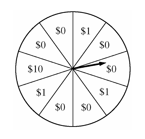
• For a payout of \$0, the net contribution is: \(\$2 – \$0 = \$2\). There are 6 sectors labeled \$0 out of 10 total sectors.
• For a payout of \$1, the net contribution is: \(\$2 – \$1 = \$1\). There are 3 sectors labeled \$1 out of 10 total sectors.
• For a payout of \$10, the net contribution is: \(\$2 – \$10 = -\$8\). There is 1 sector labeled \$10 out of 10 total sectors.
The completed probability distribution table is:

(b)
The expected value of the net contribution for a single play is calculated using the formula: \(E(X) = \sum x_i P(x_i)\).
\(E(X) = (\$2)(0.6) + (\$1)(0.3) + (-\$8)(0.1)\)
\(E(X) = 1.2 + 0.3 – 0.8\)
\(E(X) = \$0.70\)
The expected net contribution to the charity per play is \(\$0.70\).
(c)
Let \(n\) be the number of times the game is played.
The total expected net contribution for \(n\) plays is: \(E(\text{Total}) = n \cdot E(X) = 0.70n\).
We want the total expected net contribution to be at least \$500:
\(0.70n \ge 500\)
\(n \ge \dfrac{500}{0.70}\)
\(n \ge 714.29\)
Since the number of plays must be an integer, the game must be played a minimum of \(715\) times.
(d)
Let \(W\) represent the total net contribution from 1,000 plays of the game.
We are given that \(W\) is approximately normally distributed with a mean of \(\mu_W = \$700\) and a standard deviation of \(\sigma_W = \$92.79\).
We want to find the probability that the net contribution is at least \$500: \(P(W \ge 500)\).
First, compute the standardized \(z\)-score:
\(z = \dfrac{500 – \mu_W}{\sigma_W} = \dfrac{500 – 700}{92.79} = \dfrac{-200}{92.79} \approx -2.16\)
Using the standard normal probability table, the probability lying below \(z = -2.16\) is \(0.0154\).
Therefore, the probability of obtaining a net contribution of at least \$500 is:
\(P(Z \ge -2.16) = 1 – 0.0154 = 0.9846\).
The normal approximation for the probability is approximately \(0.9846\).
Question
Most-appropriate topic codes (AP Statistics):
• Topic \(2.9\) — Parameters of Random Variables (Part \(\mathrm{b}\))
▶️ Answer/Explanation
(a)
Since each question has 5 answer choices and only 1 is correct, the probability of guessing correctly on any single question is
\(p = \frac{1}{5} = 0.20\)
Each question is independent, and there are a fixed number of trials (\(n = 25\)), so \(X\) follows a binomial distribution with parameters \(n = 25\) and \(p = 0.20\):
\(X \sim B(25,\ 0.20)\)
The probability mass function is:
\(P(X = k) = \binom{25}{k}(0.20)^k(0.80)^{25-k}, \quad k = 0, 1, 2, \ldots, 25\)
Think of it this way: every question is either right or wrong (two outcomes), the questions don’t affect each other (independence), there are exactly 25 of them (fixed \(n\)), and each one has the same \(\frac{1}{5}\) chance of being correct — that’s the classic checklist for a binomial setup.
(b)
Let \(Y\) be the number of correct guesses among the 7 randomly answered questions. Then
\(Y \sim B(7,\ 0.20)\)
The expected number of correct guesses is:
\(E(Y) = np = 7 \times 0.20 = 1.4\)
Since the student answers 7 questions randomly and gets \(Y\) correct, the number answered incorrectly is \(7 – Y\). The scoring formula gives:
\(\text{Score} = (18 + Y) \times 1 – (7 – Y) \times 0.25 + 0\)
\(\text{Score} = 18 + Y – 1.75 + 0.25Y = 16.25 + 1.25Y\)
Taking the expected value:
\(E(\text{Score}) = E(16.25 + 1.25Y) = 16.25 + 1.25 \cdot E(Y)\)
\(E(\text{Score}) = 16.25 + 1.25 \times 1.4 = 16.25 + 1.75 = \boxed{18}\)
The key insight here is that even though the student is guessing on 7 questions, the penalty for wrong answers exactly offsets the expected gain from lucky correct guesses — the expected score ends up right back at 18, the number the student knew for certain.
(c)
The student passes when \(\text{Score} \geq 20\). Using the expression from part (b):
\(16.25 + 1.25Y \geq 20\)
\(1.25Y \geq 3.75\)
\(Y \geq 3\)
So the student needs to guess at least 3 of the 7 random questions correctly in order to pass. It’s easier to use the complement:
\(P(Y \geq 3) = 1 – P(Y \leq 2)\)
\(P(Y \leq 2) = P(Y=0) + P(Y=1) + P(Y=2)\)
\(= \binom{7}{0}(0.2)^0(0.8)^7 + \binom{7}{1}(0.2)^1(0.8)^6 + \binom{7}{2}(0.2)^2(0.8)^5\)
\(= (0.8)^7 + 7(0.2)(0.8)^6 + 21(0.04)(0.8)^5\)
\(= 0.2097 + 0.3670 + 0.2753\)
\(= 0.8520\)
Therefore:
\(P(Y \geq 3) = 1 – 0.8520 = \boxed{0.148}\)
There’s only about a 14.8% chance the student passes — which makes sense intuitively. Even though the expected score is exactly 18, passing requires being luckier than average on those 7 guesses, and the binomial distribution tells us that’s a relatively rare outcome.
Question

Most-appropriate topic codes (AP Statistics):
• Topic \(2.9\) — Parameters of Random Variables (Part \(\mathrm{a}\))
• Topic \(2.7\) — Independent Events and Unions of Events (Parts \(\mathrm{b}\), \(\mathrm{c}\), \(\mathrm{d}\))
▶️ Answer/Explanation
(a)
The expected value (mean) of a discrete random variable is \(\mu = \sum x_i \cdot P(x_i)\). We apply this to each player’s distribution.
For Josephine:
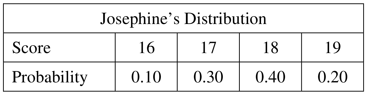
\(\mu_J = 16(0.10) + 17(0.30) + 18(0.40) + 19(0.20)\)
\(\mu_J = 1.6 + 5.1 + 7.2 + 3.8 = \boxed{17.7}\)
For Crystal:
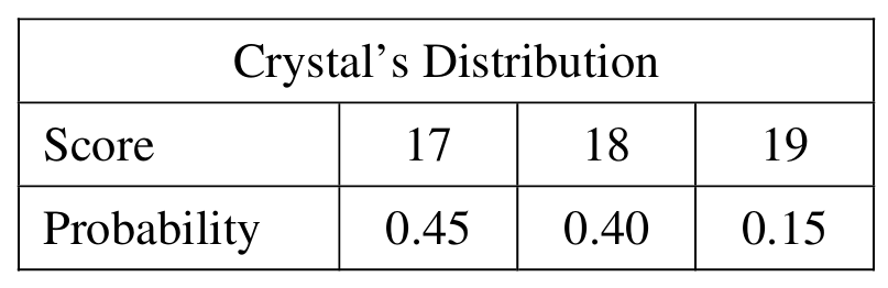
\(\mu_C = 17(0.45) + 18(0.40) + 19(0.15)\)
\(\mu_C = 7.65 + 7.20 + 2.85 = \boxed{17.7}\)
Both players have the same expected score of \(17.7\).
(b)
We need all pairs \((J, C)\) such that \(J – C = -1\), i.e., Josephine’s score is exactly 1 less than Crystal’s. Since scores are independent, the probability of each pair is the product of the individual probabilities.
\(J = 16,\ C = 17\): \(\quad P = (0.10)(0.45) = 0.045\)
\(J = 17,\ C = 18\): \(\quad P = (0.30)(0.40) = 0.120\)
\(J = 18,\ C = 19\): \(\quad P = (0.40)(0.15) = 0.060\)
These are the only three combinations that produce a difference of \(-1\).
(c)
Since the three combinations in part (b) are mutually exclusive, we simply add their probabilities:
\(P(J – C = -1) = 0.045 + 0.120 + 0.060\)
\(\boxed{P(J – C = -1) = 0.225}\)
(d)
First, we find the missing probability for a difference of \(-2\). Since all probabilities in the distribution must sum to 1:
\(P(J – C = -2) = 1 – 0.015 – 0.225 – 0.325 – 0.260 – 0.090\)
\(P(J – C = -2) = 1 – 0.915 = \boxed{0.085}\)
The completed distribution table is:

Crystal’s score is higher than Josephine’s when the difference \(J – C < 0\), i.e., when the difference is \(-3\), \(-2\), or \(-1\).
\(P(\text{Crystal} > \text{Josephine}) = P(J – C < 0) = 0.015 + 0.085 + 0.225\)
\(\boxed{P(\text{Crystal} > \text{Josephine}) = 0.325}\)
Question
Most-appropriate topic codes (AP Statistics):
• Topic 2.9 — Parameters of Random Variables (Part \(\mathrm{a}\))
• Topic 2.11 — The Normal Distribution (Parts \(\mathrm{b}\), \(\mathrm{c}\))
▶️ Answer/Explanation
(a)
Since \(X\) and \(Y\) are independent normal random variables, their difference \(Y – X\) is also normally distributed. The mean and standard deviation of \(Y – X\) are found as follows:
\(\mu_{Y-X} = \mu_Y – \mu_X = 200 – 170 = 30 \text{ minutes}\)
\(\sigma_{Y-X} = \sqrt{\sigma_Y^2 + \sigma_X^2} = \sqrt{10^2 + 20^2} = \sqrt{100 + 400} = \sqrt{500} \approx 22.36 \text{ minutes}\)
\(\boxed{Y – X \sim N(30,\ 22.36^2)}\)
The distribution of \(Y – X\) is normal with mean \(30\) minutes and standard deviation \(22.36\) minutes (variance \(500\)).
(b)
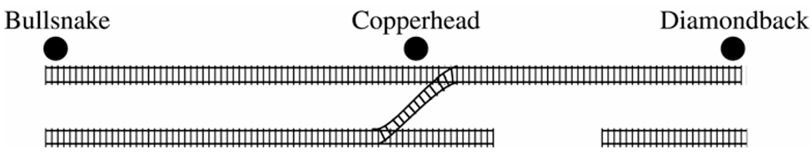
The train from Bullsnake has to wait when it arrives at Copperhead before the train from Diamondback — that is, when \(X < Y\), or equivalently when \(Y – X > 0\).
Standardize to find the \(z\)-score:
\(z = \dfrac{0 – 30}{22.36} = \dfrac{-30}{22.36} \approx -1.34\)
So the required probability is:
\(P(Y – X > 0) = P\!\left(z > -1.34\right) = 1 – P(z < -1.34) = 1 – 0.0901 = 0.9099\)
\(\boxed{P(\text{wait}) \approx 0.91}\)
About \(91\%\) of days the train from Bullsnake will have to wait at Copperhead.
(c)
Let \(D\) be the delay (in minutes) added to the Bullsnake train’s departure. The new travel-plus-delay time for the Bullsnake train is \(X + D\), where \(D\) is a constant. The difference \(Y – (X + D)\) is then normally distributed with:
\(\mu_{Y-(X+D)} = 200 – (170 + D) = 30 – D\)
\(\sigma_{Y-(X+D)} = 22.36 \text{ (unchanged, since } D \text{ is constant)}\)
We want \(P\!\left(Y – (X+D) > 0\right) = 0.01\). This means the right-tail area above \(0\) equals \(0.01\), so the left-tail area below \(0\) equals \(0.99\). The corresponding \(z\)-score for \(0.99\) is \(z = 2.33\).
Setting up the equation:
\(z = \dfrac{0 – (30 – D)}{22.36} = 2.33\)
\(0 – (30 – D) = 2.33 \times 22.36\)
\(D – 30 = 52.10\)
\(D = 82.10 \text{ minutes}\)
\(\boxed{D \approx 82 \text{ minutes}}\)
The Snake Gulch Railroad should delay the departure of the train from Bullsnake by approximately \(82\) minutes so that the probability of having to wait drops to only \(0.01\).
Question

Most-appropriate topic codes (AP Statistics):
• Topic 2.12 — Sampling Distributions and the Central Limit Theorem (Part \(\mathrm{b}\))
• Topic 1.7 — Summary Statistics for One Quantitative Variable (Part \(\mathrm{c}\))
• Topic 1.9 — Comparisons of the Distributions for One Quantitative Variable (Part \(\mathrm{d}\))
▶️ Answer/Explanation
(a)
The expected value of a discrete random variable is found by multiplying each value by its probability and adding the results:
\( E(X)=\sum x_i\,p(x_i) \)
Plugging in the values from the table:
\( E(X)=0(0.35)+1(0.20)+2(0.15)+3(0.15)+4(0.10)+5(0.05) \)
\( E(X)=0+0.20+0.30+0.45+0.40+0.25 \)
\( \boxed{E(X)=1.6} \)
(b)
Both sample averages are estimates of the same population mean, \(\mu_X=1.6\), so they should be centered around the same value. What changes is how precise that estimate is.
The standard deviation of a sample mean is
\( \sigma_{\bar{x}}=\dfrac{\sigma}{\sqrt{n}} \)
Since \(1{,}000>20\), a sample of 1,000 days has a much smaller standard deviation for its average, meaning the sample average will tend to land closer to 1.6 than the first sample’s average of 1.25 did.
\( \boxed{\text{The new average should be closer to } 1.6\text{ than }1.25\text{, since larger samples have less variability}} \)
(c)
To find the median, build up the cumulative probabilities:
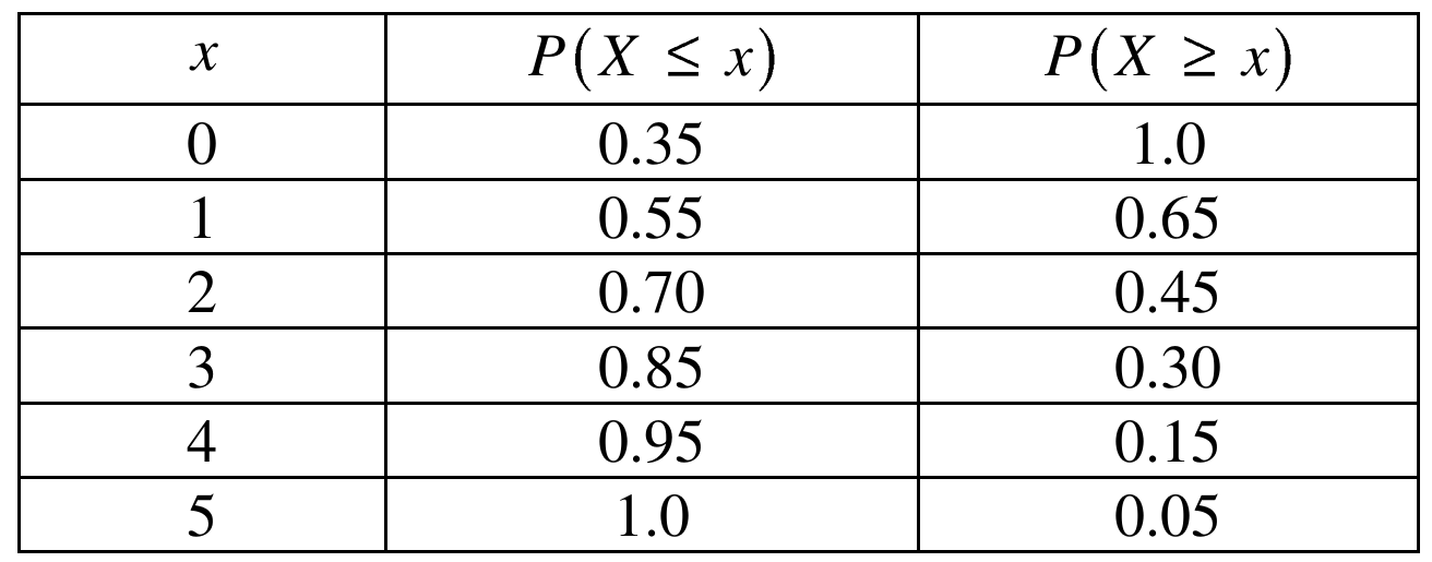
At \(x=1\), both \(P(X\le 1)=0.55\ge 0.5\) and \(P(X\ge 1)=0.65\ge 0.5\) are satisfied. At \(x=2\), \(P(X\ge 2)=0.45<0.5\), so \(x=2\) does not work.
\( \boxed{\text{Median} = 1} \)
(d)
Looking at the table, most of the probability is piled up at the small values (0, 1, 2) with a long tail of smaller probabilities stretching out to 4 and 5. This makes the distribution right-skewed, which pulls the mean up above the median — here the mean of 1.6 is noticeably larger than the median of 1, which is exactly the pattern you’d expect for a distribution skewed toward larger values.
\( \boxed{\text{The distribution is right-skewed, so the mean (1.6) is greater than the median (1)}} \)
Question
Most-appropriate topic codes (AP Statistics):
• Topic 2.9 — Parameters of Random Variables (Parts a, b, c)
▶️ Answer/Explanation
(a)
The mean of a discrete random variable is computed by multiplying each value by its probability and summing:
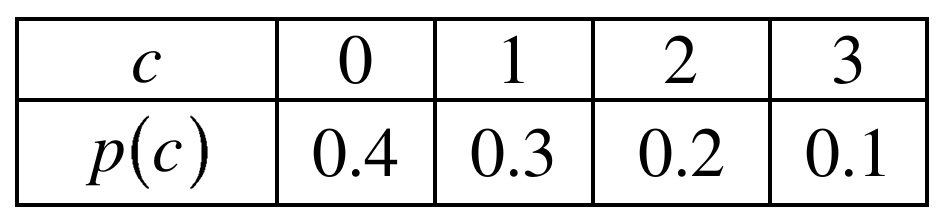
\( \mu_C = \sum c \cdot p(c) = (0)(0.4) + (1)(0.3) + (2)(0.2) + (3)(0.1) \)
\( \mu_C = 0 + 0.3 + 0.4 + 0.3 = \boxed{1} \)
For the standard deviation, first compute the variance using \(\sigma_C^2 = \sum (c – \mu_C)^2 \cdot p(c)\):
\( \sigma_C^2 = (0-1)^2(0.4) + (1-1)^2(0.3) + (2-1)^2(0.2) + (3-1)^2(0.1) \)
\( \sigma_C^2 = (1)(0.4) + (0)(0.3) + (1)(0.2) + (4)(0.1) = 0.4 + 0 + 0.2 + 0.4 = 1 \)
Taking the square root gives the standard deviation:
\( \boxed{\sigma_C = \sqrt{1} = 1} \)
It’s a neat coincidence here that the variance and standard deviation are both equal to 1 — don’t mix them up!
(b)
Let \(T = C + A\), where \(A\) is the number of adult tickets purchased. We are given \(\mu_A = 2\) and \(\sigma_A = 1.2\).
Since means always add regardless of independence:
\( \mu_T = \mu_C + \mu_A = 1 + 2 = \boxed{3} \)
Because \(C\) and \(A\) are independent, variances add (not standard deviations):
\( \sigma_T^2 = \sigma_C^2 + \sigma_A^2 = (1)^2 + (1.2)^2 = 1 + 1.44 = 2.44 \)
\( \sigma_T = \sqrt{2.44} \approx \boxed{1.562} \)
Remember: you can only add variances directly when the variables are independent — never add the standard deviations themselves.
(c)
Let \(M = 15C + 25A\) be the total amount spent per purchase.
For the mean, use the linearity of expectation:
\( \mu_M = 15\,\mu_C + 25\,\mu_A = 15(1) + 25(2) = 15 + 50 = \boxed{\$65} \)
For the variance, when scaling a random variable by a constant \(k\), the variance scales by \(k^2\). Since \(C\) and \(A\) are independent:
\( \sigma_M^2 = (15)^2\,\sigma_C^2 + (25)^2\,\sigma_A^2 = 225(1) + 625(1.44) \)
\( \sigma_M^2 = 225 + 900 = 1125 \)
\( \sigma_M = \sqrt{1125} \approx \boxed{\$33.54} \)
The key idea here is that multiplying a random variable by a constant multiplies its standard deviation by that constant, but you still must add variances (not standard deviations) when combining two independent variables.
Question
Most-appropriate topic codes (AP Statistics):
• Topic 2.8 — Introduction to Random Variables and Probability Distributions (Part b)
• Topic 2.9 — Parameters of Random Variables (Parts b, c)
▶️ Answer/Explanation
(a)
Under Plan I, a child is cured if antibiotic A works, or if A fails but antibiotic B then works. Since the antibiotics act independently:
\(P(\text{cured} \mid \text{Plan I}) = P(A \text{ cures}) + P(A \text{ fails}) \times P(B \text{ cures})\)
\(= 0.60 + (0.40)(0.90)\)
\(= 0.60 + 0.36\)
\(\boxed{P(\text{cured} \mid \text{Plan I}) = 0.96}\)
Under Plan II, a child is cured if antibiotic B works, or if B fails but antibiotic A then works:
\(P(\text{cured} \mid \text{Plan II}) = P(B \text{ cures}) + P(B \text{ fails}) \times P(A \text{ cures})\)
\(= 0.90 + (0.10)(0.60)\)
\(= 0.90 + 0.06\)
\(\boxed{P(\text{cured} \mid \text{Plan II}) = 0.96}\)
Both plans result in the same probability of curing the infection: \(0.96\).
(b)
For Plan I, there are two possible treatment scenarios:
— Antibiotic A cures the child (probability \(0.60\)): cost \(= \$50\)
— Antibiotic A fails, then antibiotic B is administered (probability \(0.40\)): cost \(= \$50 + \$80 = \$130\)
\(E(\text{cost} \mid \text{Plan I}) = (0.60)(\$50) + (0.40)(\$130)\)
\(= \$30 + \$52\)
\(\boxed{E(\text{cost} \mid \text{Plan I}) = \$82}\)
For Plan II, there are two possible treatment scenarios:
— Antibiotic B cures the child (probability \(0.90\)): cost \(= \$80\)
— Antibiotic B fails, then antibiotic A is administered (probability \(0.10\)): cost \(= \$80 + \$50 = \$130\)
\(E(\text{cost} \mid \text{Plan II}) = (0.90)(\$80) + (0.10)(\$130)\)
\(= \$72 + \$13\)
\(\boxed{E(\text{cost} \mid \text{Plan II}) = \$85}\)
(c)
Plan I is the better recommendation. Both plans produce identical probabilities of curing the infection (\(0.96\)), so neither plan has an advantage in terms of treatment effectiveness. However, Plan I has a lower expected cost per child (\(\$82\)) compared to Plan II (\(\$85\)). Since the insurance company is equally likely to achieve a cure under either plan but will spend \(\$3\) less per child on average under Plan I, recommending Plan I is the more cost-effective choice.
\(\boxed{\text{Recommend Plan I: same cure probability (0.96), lower expected cost (\$82 vs. \$85)}}\)
Question
Most-appropriate topic codes (AP Statistics):
• Topic 3.3 — Constructing a Confidence Interval for a Population Proportion (Part b)
• Topic 3.4 — Justifying a Claim Based on a Confidence Interval for a Population Proportion (Parts c, d)
▶️ Answer/Explanation
(a)
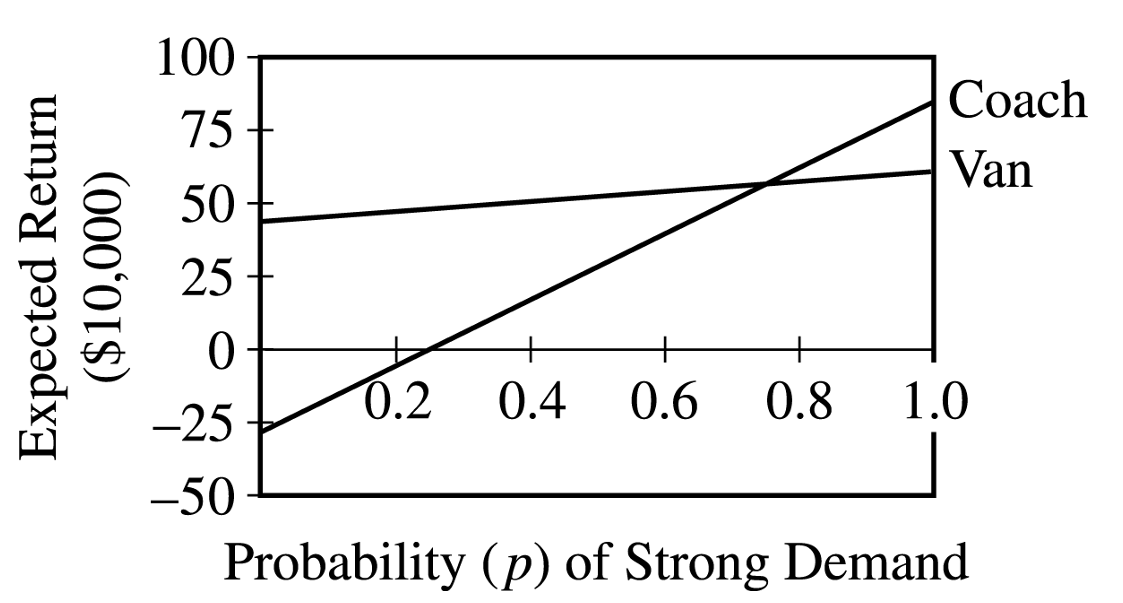
Looking at the graph, the line for vans starts higher than the line for coaches when \(p\) is small (since vans don’t lose much money even in a weak market), but the coach line rises more steeply and eventually overtakes the van line at \(p=0.76\). For any \(p\) less than \(0.76\), the van line sits above the coach line, meaning vans give the larger expected return.
We can also confirm this algebraically by plugging in a value of \(p\) less than \(0.76\), say \(p=0.5\):
Expected return for coaches:
\( 111(0.5)-27=55.5-27=28.5 \)
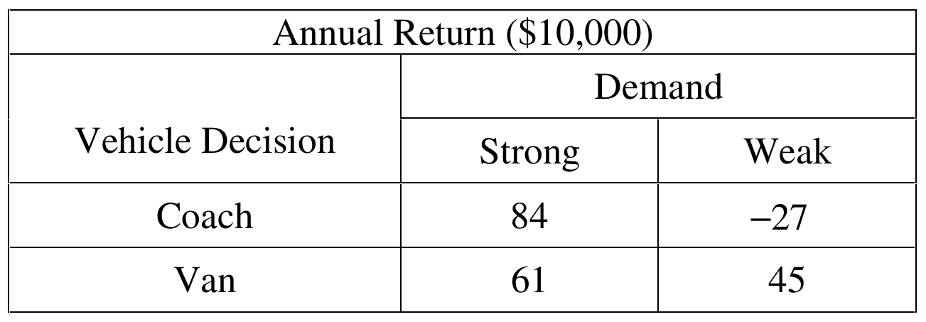
So the coach return is \(\$285{,}000\).
Expected return for vans:
\( 16(0.5)+45=8+45=53 \)
So the van return is \(\$530{,}000\).
Since \(53>28.5\), vans give the higher expected return at \(p=0.5\). Because both expected-return equations are linear in \(p\) and the two lines cross only once (at \(p=0.76\)), this same ordering — vans above coaches — must hold for every value of \(p\) below \(0.76\).
\( \boxed{\text{For } p<0.76, \text{ vans provide the greater expected annual return.}} \)
(b)
Since we’re estimating the proportion \(p\) of similar markets with strong demand based on a sample proportion, this calls for a one-sample \(z\)-confidence interval for a proportion.
From the sample,
\( \hat{p}=\dfrac{65}{100}=0.65 \)
Before building the interval, check the conditions. The \(100\) markets were a random sample, and since there are several thousand similar markets nationally, \(100\) is less than \(10\%\) of that population. For the large-sample condition,
\( n\hat{p}=100(0.65)=65 \)
\( n(1-\hat{p})=100(0.35)=35 \)
Both of these are well above \(10\), so a normal approximation is reasonable and the interval can proceed.
The formula for the confidence interval is:
\( \hat{p}\pm z^{*}\sqrt{\dfrac{\hat{p}(1-\hat{p})}{n}} \)
Compute the standard error first:
\( \sqrt{\dfrac{(0.65)(0.35)}{100}}=\sqrt{\dfrac{0.2275}{100}}=\sqrt{0.002275} \)
\( \approx0.0477 \)
For \(95\%\) confidence, \(z^{*}=1.96\), so the margin of error is:
\( 1.96\times0.0477\approx0.0935 \)
Putting it together:
\( 0.65\pm0.0935 \)
\( \boxed{(0.5565,\ 0.7435)} \)
Interpretation: We can be \(95\%\) confident that the true proportion of similar markets that will experience strong demand is between about \(0.56\) and \(0.74\).
(c)
The interval from part (b) tells us that the plausible values for \(p\), the probability of strong demand, range from about \(0.56\) to \(0.74\). Every single value in that interval is less than \(0.76\), the cutoff found in part (a). Since part (a) showed that vans produce a larger expected return than coaches whenever \(p<0.76\), this means that for every plausible value of \(p\) suggested by the data, vans come out ahead. So choosing vans makes sense — it’s the decision that’s expected to perform better across the entire range of demand probabilities that the sample data support.
(d)
Even though the entire confidence interval lies below \(0.76\), the vice president could argue based on the actual dollar amounts at stake rather than just which option has the slightly higher expected return. Notice that throughout the confidence interval \((0.56,\ 0.74)\), the probability of strong demand is consistently estimated to be greater than \(0.5\) — meaning strong demand is more likely than weak demand in this market.
If demand turns out to be strong, the payoff table shows coaches return \(\$840{,}000\) compared to only \(\$610{,}000\) for vans — a substantial difference in the company’s favor. Meanwhile, if demand is weak, coaches lose \(\$270{,}000\) while vans still make \(\$450{,}000\), but this weak-demand scenario is the less likely one according to the interval. So the vice president could reasonably argue that, since strong demand is more probable and the upside for coaches in that case is so much larger than the modest expected-value edge vans have overall, coaches are actually the better choice for this particular route.
Question
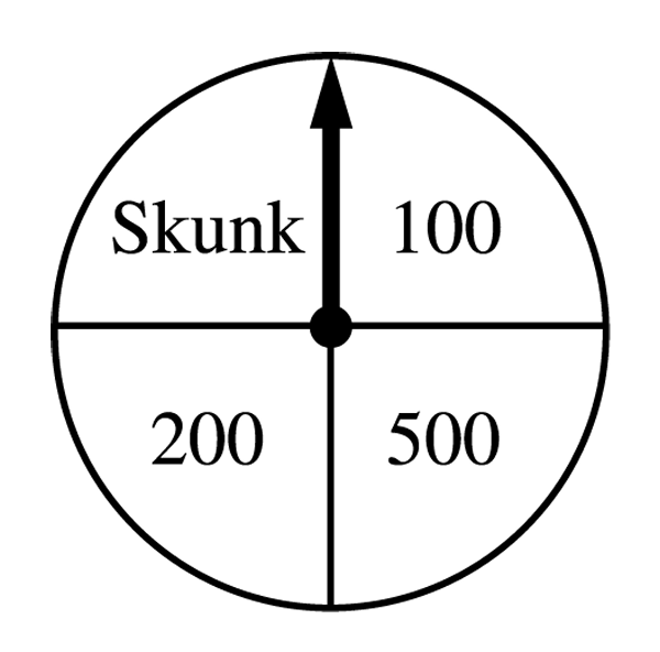
- The contestant spins the wheel.
- If the result is a skunk, no money is won and the contestant’s turn is finished.
- If the result is a number, the corresponding amount in dollars is won. The contestant can then stop with those winnings or can choose to spin again, and his or her turn continues.
- If the contestant spins again and the result is a skunk, all of the money earned on that turn is lost and the turn ends.
- The contestant may continue adding to his or her winnings until he or she chooses to stop or until a spin results in a skunk.

Most-appropriate topic codes (AP Statistics):
• Topic 2.9 — Parameters of Random Variables (Part b)
• Topic 3.14 — Setting Up a Chi-Square Test for Homogeneity or Independence (Part c)
• Topic 3.15 — Carrying Out a Chi-Square Test for Homogeneity or Independence (Part c)
▶️ Answer/Explanation
(a)
There are four equally likely outcomes on the wheel: Skunk, \(\$100\), \(\$200\), and \(\$500\). So the probability of landing on a number (i.e., not a skunk) on any single spin is \(\dfrac{3}{4}\).
Since spins are independent, the probability of getting a number on all three of the first three spins is:
\( P(\text{number on all 3 spins}) = \left(\frac{3}{4}\right)^3 = \frac{27}{64} \approx 0.4219 \)
\(\boxed{P \approx 0.4219}\)
(b)
The contestant currently has \(\$800\) and chooses to spin a fourth time. The four equally likely outcomes on the fourth spin lead to the following total winnings:
The expected value of total winnings is:
\( E(\text{total winnings}) = 0\left(\frac{1}{4}\right) + 900\left(\frac{1}{4}\right) + 1000\left(\frac{1}{4}\right) + 1300\left(\frac{1}{4}\right) \)
\( = \frac{0 + 900 + 1000 + 1300}{4} = \frac{3200}{4} = \$800 \)
Alternatively, the expected gain from the fourth spin alone is:
\( E(\text{4th spin gain}) = (-800)\left(\frac{1}{4}\right) + 100\left(\frac{1}{4}\right) + 200\left(\frac{1}{4}\right) + 500\left(\frac{1}{4}\right) = \frac{-800+100+200+500}{4} = 0 \)
So the expected total winnings \(= \$800 + \$0 = \boxed{\$800}\).
Interestingly, the expected value of spinning again is exactly equal to the amount already won — so on average the fourth spin neither helps nor hurts.
(c)
Hypotheses:
\( H_0: p_1 = p_2 = p_3 = p_4 = \frac{1}{4} \quad \text{(all four outcomes are equally likely)} \)
\( H_a: \text{at least one } p_i \neq \frac{1}{4} \quad \text{(the four outcomes are not equally likely)} \)
Test: Chi-square goodness-of-fit test.
Conditions: The spins are independent (stated in the problem), and the expected count for each outcome is \(100 \times \frac{1}{4} = 25 > 5\), so the sample size is large enough to proceed.
Expected counts: 25 for each of the four outcomes.
Test statistic:
\( \chi^2 = \sum \frac{(\text{Observed} – \text{Expected})^2}{\text{Expected}} \)
\( = \frac{(33-25)^2}{25} + \frac{(21-25)^2}{25} + \frac{(20-25)^2}{25} + \frac{(26-25)^2}{25} \)
\( = \frac{64}{25} + \frac{16}{25} + \frac{25}{25} + \frac{1}{25} = \frac{106}{25} = 4.24 \)
Degrees of freedom: \(df = 4 – 1 = 3\)
P-value: \(p\text{-value} \approx 0.237\) (from chi-square table with \(df = 3\), the test statistic of 4.24 falls well below the critical value of 7.81 at \(\alpha = 0.05\)).
Conclusion: Since the \(p\text{-value} \approx 0.237 > 0.05\), we fail to reject \(H_0\). There is not convincing statistical evidence that the four outcomes on the wheel are not equally likely — the data are consistent with a fair wheel.