
AP Statistics 3.1 Estimators- Exam Style Questions - FRQs - New Syllabus
Question
Most-appropriate topic codes (AP Statistics):
• Topic \(3.10\) — Constructing a Confidence Interval for the Difference Between Two Population Proportions (Part \(\mathrm{b}\))
• Topic \(3.11\) — Justifying a Claim Based on a Confidence Interval for the Difference Between Two Population Proportions (Parts \(\mathrm{b}\), \(\mathrm{e}\))
• Topic \(3.1\) — Estimators (Part \(\mathrm{c}\): estimating relative risk using \(\hat{p}_A/\hat{p}_B\))
• Topic \(3.11\) — Justifying a Claim Based on a Confidence Interval for the Difference Between Two Population Proportions (Part \(\mathrm{d}\): interpreting the confidence interval for relative risk)
▶️ Answer/Explanation
(a)
Yes, this experiment can be performed as a double-blind experiment by introducing placebos for each treatment group.
Patients assigned to treatment A (pill) would also receive a placebo injection. Patients assigned to treatment B (injection) would also receive a placebo pill. This way, every patient receives both a pill and an injection, but one of the two is a placebo.
Since neither the patients nor the physicians administering the treatments know which is the real treatment and which is the placebo, neither group is aware of the treatment assignment — making the experiment double-blind.
(b)
First, compute the sample proportions:
\(\hat{p}_A = \frac{38}{154} \approx 0.2468, \qquad \hat{p}_B = \frac{16}{164} \approx 0.0976\)
The 95% confidence interval for \(p_A – p_B\) is:
\(\hat{p}_A – \hat{p}_B) \pm z^* \sqrt{\frac{\hat{p}_A(1-\hat{p}_A)}{n_A} + \frac{\hat{p}_B(1-\hat{p}_B)}{n_B}}\)
\(0.2468 – 0.0976) \pm 1.96\sqrt{\frac{(0.2468)(0.7532)}{154} + \frac{(0.0976)(0.9024)}{164}}\)
\(0.1492 \pm 1.96(0.0418)\)
\(0.1492 \pm 0.0818\)
\(\boxed{(0.0674,\ 0.2310)}\)
We are 95% confident that the true difference in 15-year survival rates \((p_A – p_B)\) is between \(0.0674\) and \(0.2310\). Because the entire interval lies above zero, this provides evidence that treatment A has a higher 15-year survival rate than treatment B.
(c)
The estimated relative risk is:
\(\frac{\hat{p}_A}{\hat{p}_B} = \frac{38/154}{16/164} = \frac{0.2468}{0.0976} \approx 2.53\)
\(\boxed{\text{Estimated relative risk} \approx 2.53}\)
This means patients receiving treatment A are estimated to be about 2.53 times as likely to survive at least 15 years as patients receiving treatment B.
(d)
A 95% confidence interval for \(\ln\!\left(\dfrac{p_A}{p_B}\right)\) is given as \((0.3868,\ 1.4690)\).
To convert this to a confidence interval for the relative risk \(\dfrac{p_A}{p_B}\), apply the exponential (inverse of the natural log) to each endpoint:
\(e^{0.3868} \approx 1.47 \qquad \text{and} \qquad e^{1.4690} \approx 4.34\)
\(\boxed{\left(1.47,\ 4.34\right)}\)
We are 95% confident that patients receiving treatment A are between 1.47 and 4.34 times as likely to survive at least 15 years compared to patients receiving treatment B.
(e)
When the survival proportions are small (as here, approximately 0.25 and 0.10), the confidence interval for the relative risk is more informative and practically meaningful than the confidence interval for the difference in proportions.
Knowing that a patient’s chance of survival is between 1.47 and 4.34 times greater with treatment A is more vivid and easier to interpret clinically than knowing the absolute difference in proportions is somewhere between 0.07 and 0.23 — a range that may sound small even though it represents a substantial relative advantage.
Question
Most-appropriate topic codes (AP Statistics):
• Topic \(1.7\) — Summary Statistics for a Quantitative Variable (Center, Spread, Shape) (Parts \(\mathrm{a}\), \(\mathrm{b}\), \(\mathrm{c}\))
• Topic \(1.9\) — Comparing Distributions of a Quantitative Variable (Parts \(\mathrm{a}\), \(\mathrm{b}\))
• Topic \(1.10\) — The Effect of Adding a Constant or Multiplying by a Constant on Summary Statistics (Part \(\mathrm{b}\))
• Topic \(3.1\) — Mean and Standard Deviation of a Linear Transformation (Part \(\mathrm{c}\))
▶️ Answer/Explanation
(a)
When comparing two distributions from boxplots, we examine center, spread, shape, and unusual features.
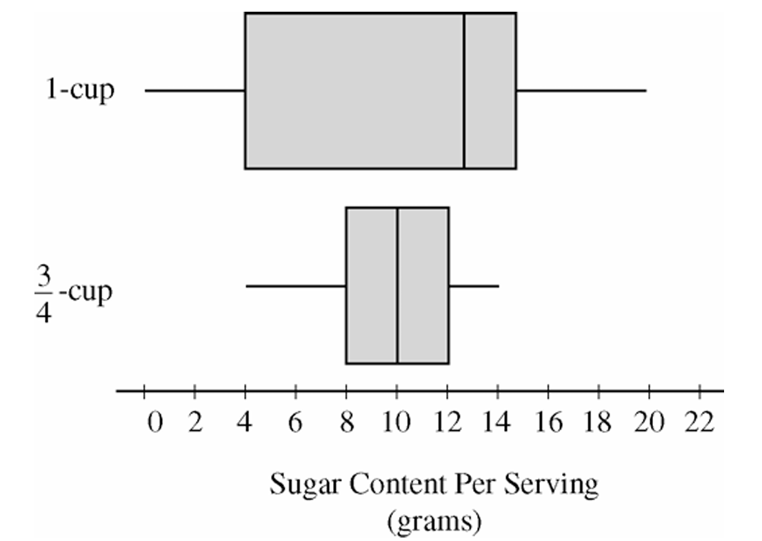
The cereals with one-cup serving sizes have a higher median sugar content per serving than the cereals with three-quarter-cup serving sizes. The one-cup distribution also has greater variability, as indicated by its larger range and larger interquartile range (IQR). In terms of shape, the one-cup distribution appears somewhat left-skewed because the median is closer to the upper quartile than to the lower quartile, while the three-quarter-cup distribution is more nearly symmetric. Neither distribution appears to contain extreme outliers.
(b)
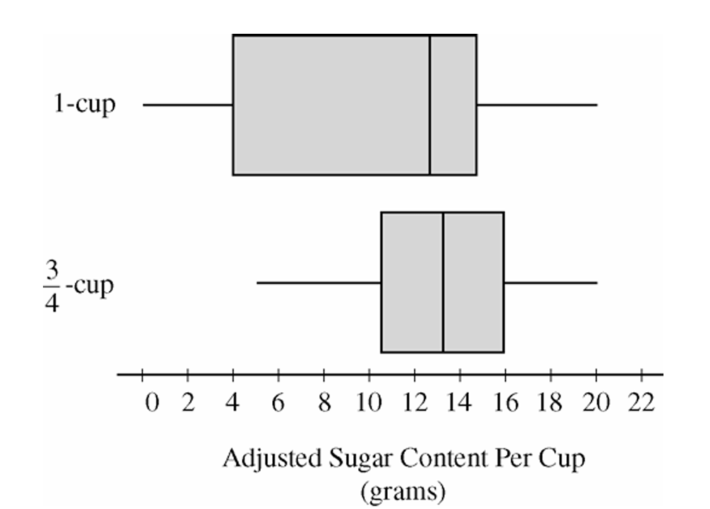
Multiplying each sugar value in the three-quarter-cup group by \(\dfrac{4}{3}\) converts the measurements to sugar content per cup, allowing a fair comparison using equal serving sizes.
The adjusted boxplot shows that cereals with recommended serving sizes of three-quarter cup tend to contain more sugar per cup than cereals with recommended serving sizes of one cup. The median for the adjusted three-quarter-cup distribution is now noticeably higher than the median for the one-cup distribution. In addition, all measures of spread (range and IQR) for the adjusted distribution have increased by a factor of \(\dfrac{4}{3}\), reflecting the effect of multiplying every observation by a constant.
(c)
We would expect the mean sugar content per cup to be greater for cereals that list a serving size of three-quarter cup.
After adjustment, the three-quarter-cup distribution has a higher center than the one-cup distribution, as seen from its higher median. Because the mean generally follows the center of the distribution, the higher overall location of the adjusted three-quarter-cup distribution suggests a larger mean sugar content per cup.
\(\boxed{\bar{x}_{\frac{3}{4}\text{-cup}} > \bar{x}_{\text{1-cup}}}\)
Question
How can you tell?
Explain your choice.
Explain your choice.
Most-appropriate topic codes (AP Statistics):
• Topic 2.12 — Sampling Distributions and the Central Limit Theorem (Part \(\mathrm{a}\))
▶️ Answer/Explanation
(a)
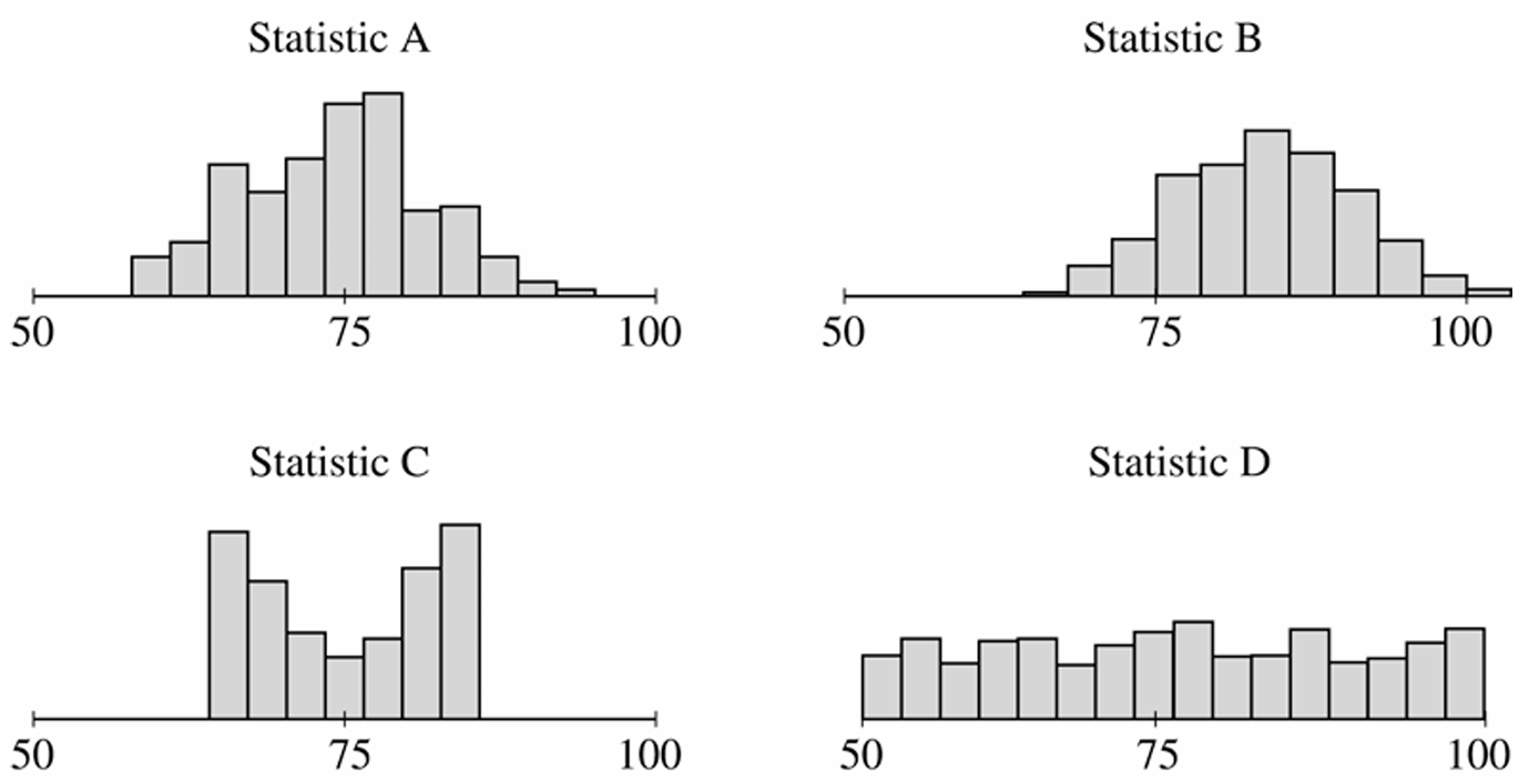
Statistics \(A\), \(C\), and \(D\) appear to be unbiased estimators of the population parameter.
An estimator is said to be unbiased if the mean (center) of its sampling distribution equals the true population parameter. In other words, there is no systematic tendency to overestimate or underestimate.
For Statistics \(A\), \(C\), and \(D\), the distributions appear to be centered at approximately \(\mu_{\text{stat}} \approx 75\), which equals the true population parameter value of \(75\).
For Statistic \(B\), the distribution is centered at approximately \(85\), which is clearly greater than \(75\), so Statistic \(B\) is a biased estimator — it consistently overestimates the parameter.
\(\boxed{\text{Unbiased estimators: Statistics } A,\ C,\ \text{and } D}\)
(b)
Statistic \(A\) would be the better estimator between \(A\) and \(B\).
Statistic \(B\) is centered at approximately \(85\), which is far from the true parameter value of \(75\) — it is a biased estimator that systematically overestimates.
Statistic \(A\), on the other hand, is centered at approximately \(75\), making it an unbiased estimator. Both \(A\) and \(B\) have roughly similar variability (spread), but since only \(A\) is centered at the true parameter, \(A\) will consistently produce estimates closer to \(75\).
\(\boxed{\text{Statistic } A \text{ is the better estimator}}\)
(c)
Statistic \(C\) would be the better estimator between \(C\) and \(D\).
Both Statistics \(C\) and \(D\) appear to be unbiased — their distributions are each centered at approximately \(75\), the true population parameter value. So bias is not a distinguishing factor here.
However, the two differ substantially in variability. Statistic \(C\) has a much smaller spread (lower variance), meaning its estimates cluster tightly around \(75\). Statistic \(D\) has a very large spread, so its individual estimates can deviate far from \(75\), even though on average they are correct.
Since both estimators are unbiased, the one with lower variability is preferred — it will produce more precise estimates in practice.
\(\boxed{\text{Statistic } C \text{ is the better estimator}}\)
Question
Most-appropriate topic codes (AP Statistics):
• Topic 3.15 — Carrying Out a Chi-Square Test for Homogeneity or Independence (Part a)
• Topic 3.1 — Estimators (Part b)
• Topic 1.11 — Random Sampling (Part b)
▶️ Answer/Explanation
(a)
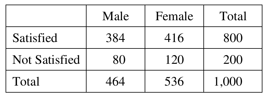
The appropriate procedure is a chi-square test for independence.
Hypotheses:
\(H_0\): Gender and satisfaction with hospital services are independent (no association).
\(H_a\): Gender and satisfaction with hospital services are not independent (there is an association)
Conditions:
— The sample is a random sample of 1,000 adult county residents.
— All expected cell counts must be at least 5.
Compute each:
\(E = \frac{(\text{row total})(\text{column total})}{\text{grand total}}\)
\(E(\text{Satisfied, Male}) = \dfrac{800 \times 464}{1000} = 371.2\)
\(E(\text{Satisfied, Female}) = \dfrac{800 \times 536}{1000} = 428.8\)
\(E(\text{Not Satisfied, Male}) = \dfrac{200 \times 464}{1000} = 92.8\)
\(E(\text{Not Satisfied, Female}) = \dfrac{200 \times 536}{1000} = 107.2\)
All expected counts are well above 5.
Test Statistic:
\(\chi^2 = \sum \frac{(O – E)^2}{E}\)
\(\chi^2 = \frac{(384 – 371.2)^2}{371.2} + \frac{(416 – 428.8)^2}{428.8} + \frac{(80 – 92.8)^2}{92.8} + \frac{(120 – 107.2)^2}{107.2}\)
\(\chi^2 = \frac{(12.8)^2}{371.2} + \frac{(-12.8)^2}{428.8} + \frac{(-12.8)^2}{92.8} + \frac{(12.8)^2}{107.2}\)
\(\chi^2 = 0.4413 + 0.3821 + 1.7655 + 1.5284 = 4.117\)
Degrees of freedom:
\(df = (r-1)(c-1) = (2-1)(2-1) = 1\)
P-value:
Using the \(\chi^2\) distribution with \(df = 1\):
\(p\text{-value} \approx 0.0424\)
Conclusion:
Since \(p\text{-value} = 0.0424 < \alpha = 0.05\), we reject \(H_0\). There is sufficient statistical evidence at the \(0.05\) significance level to conclude that there is an association between gender and satisfaction with hospital services for adult residents of this county.
\(\boxed{\chi^2 = 4.117,\quad df = 1,\quad p\text{-value} \approx 0.0424 \Rightarrow \text{Reject } H_0}\)
(b)
Yes, \(\dfrac{800}{1{,}000} = 0.80\) is a reasonable estimate for the proportion of all adult county residents who are satisfied with hospital services. The data were collected from a random sample of 1,000 adult county residents, which means the sample is likely representative of the population of all adult county residents. Because random sampling was used, the sample proportion \(\hat{p} = 0.80\) is an unbiased estimate of the true population proportion. Additionally, with a sample size of \(n = 1{,}000\), the estimate is based on a sufficiently large and randomly selected group, giving us reasonable confidence in its accuracy.
\(\boxed{\hat{p} = \frac{800}{1{,}000} = 0.80 \text{ is a reasonable estimate (random sample, large } n\text{)}}\)
Question
Most-appropriate topic codes (AP Statistics):
• Topic 3.13 — Carrying Out a Test for the Difference Between Two Population Proportions (Part a)
• Topic 3.1 — Estimators (Part b)
• Topic 1.11 — Random Sampling (Part c)
• Topic 1.12 — Potential Problems with Sampling (Part c)
▶️ Answer/Explanation
(a)
Step 1: State hypotheses.
Let \(p_A\) = true proportion of banded birds on Island A, and \(p_B\) = true proportion of banded birds on Island B.
\(H_0: p_A – p_B = 0 \qquad H_a: p_A – p_B \neq 0\)
Step 2: Identify the test and check assumptions.
We use a two-sample \(z\)-test for a difference in proportions. The test statistic is:
\(z = \dfrac{\hat{p}_A – \hat{p}_B}{\sqrt{\hat{p}(1-\hat{p})\left(\dfrac{1}{n_1} + \dfrac{1}{n_2}\right)}}\)
The problem states the samples are random. Since the two islands are separate, the samples are independent. We check the large sample condition using the pooled estimate:
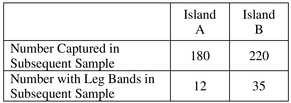
\(\hat{p} = \dfrac{n_A\hat{p}_A + n_B\hat{p}_B}{n_A + n_B} = \dfrac{12 + 35}{180 + 220} = \dfrac{47}{400} = 0.1175\)
Expected counts: \(n_A\hat{p} = 21.15,\quad n_A(1-\hat{p}) = 158.85,\quad n_B\hat{p} = 25.85,\quad n_B(1-\hat{p}) = 194.15\)
All expected counts are well above 5, so the large sample condition is satisfied.
Step 3: Compute the test statistic and p-value.
\(\hat{p}_A = \dfrac{12}{180} = 0.067 \qquad \hat{p}_B = \dfrac{35}{220} = 0.159\)
\(z = \dfrac{0.067 – 0.159}{\sqrt{\dfrac{(0.1175)(0.8825)}{180} + \dfrac{(0.1175)(0.8825)}{220}}} = \dfrac{-0.092}{\sqrt{0.00105}} = \dfrac{-0.092}{0.032} = -2.875\)
\(\text{p-value} = 2 \times P(Z < -2.875) \approx 0.00429\)
Step 4: State conclusion in context.
Since the p-value of \(0.00429\) is less than \(\alpha = 0.05\), we reject the null hypothesis. There is convincing statistical evidence that the proportions of banded birds on the two islands are different — Island B has a notably higher proportion of banded birds than Island A.
(b)
We use the capture-recapture logic: the proportion of banded birds in the subsequent sample estimates the proportion of banded birds in the whole population.
For Island A, the number of birds banded in the initial sample is \(n_I = 200\), and the proportion of banded birds observed in the subsequent sample is:
\(\hat{p}_S = \dfrac{12}{180} \approx 0.06667\)
Setting this equal to the fraction of banded birds in the population:
\(\hat{p}_S \approx \dfrac{n_I}{\text{population size}}\)
Solving for the estimated population size:
\(\text{Estimated population size} = \dfrac{n_I}{\hat{p}_S} = \dfrac{200}{12/180} = \dfrac{200 \times 180}{12} = \dfrac{36{,}000}{12} = \boxed{3{,}000 \text{ birds}}\)
(c)
Two concerns that should be addressed before assuming the captures can be treated as random samples are:
Concern 1 — Differential catchability: Some birds may be more likely to be captured than others — for example, slower, older, or less wary birds might be caught at a higher rate than the general population. If the same birds that were easy to capture in the initial sample are also more likely to appear in the subsequent sample, then banded birds would be overrepresented in the subsequent sample, leading us to underestimate the true population size.
Concern 2 — Behavioural change after banding: Birds that were captured and banded in the initial sample may become more trap-shy (avoiding capture in the future) or, conversely, may be more conspicuous to predators due to the bands, altering their survival or behaviour. If banded birds are less likely to be recaptured, we would overestimate the population size. In either case, if banding changes the birds’ behaviour or survival, the subsequent sample can no longer be treated as a true random sample of the population.
Question

Most-appropriate topic codes (AP Statistics):
• Topic 3.4 — Justifying a Claim Based on a Confidence Interval for a Population Proportion (Part a)
• Topic 3.1 — Estimators (Part b)
• Topic 3.2 — Sampling Distributions for Sample Proportions (Parts b, c)
▶️ Answer/Explanation
(a)
Procedure and Conditions:
We use a one-sample \(z\)-confidence interval for a proportion: \(\hat{p} \pm z^* \sqrt{\dfrac{\hat{p}(1-\hat{p})}{n}}\).
From the table, the sample of females in the 40–44 age-group has \(n = 370\). With 10% contracting the illness, \(\hat{p} = 0.10\).
Check conditions: The sample is a random sample from the HMO population. The expected number of successes is \(n\hat{p} = 370(0.10) = 37 > 5\) and the expected number of failures is \(n(1-\hat{p}) = 370(0.90) = 333 > 5\), so the sample size is large enough to proceed.
Mechanics:
\( \hat{p} \pm z^* \sqrt{\frac{\hat{p}(1-\hat{p})}{n}} = 0.10 \pm 1.96\sqrt{\frac{(0.10)(0.90)}{370}} \)
\( = 0.10 \pm 1.96\sqrt{\frac{0.09}{370}} = 0.10 \pm 1.96(0.01559) = 0.10 \pm 0.0306 \)
\( \boxed{(0.06943,\ 0.13057)} \)
Interpretation of the confidence interval:
We are 95% confident that the true proportion of the HMO’s 40–44 year old female patients who would contract this illness is between approximately 0.069 and 0.131 (i.e., between about 6.9% and 13.1%).
Interpretation of the 95% confidence level:
If we were to take many random samples of size 370 from this population and compute a 95% confidence interval from each sample, approximately 95% of those intervals would capture the true population proportion of 40–44 year old female HMO patients who contract the illness. In other words, the method we used to construct this interval will fail to contain the true proportion only about 5% of the time in repeated sampling.
(b)
The width of a confidence interval for a proportion is determined by the margin of error \(z^*\sqrt{\dfrac{\hat{p}(1-\hat{p})}{n}}\), which depends on both \(\hat{p}\) and \(n\).
When the sample proportions are equal (both 0.10), the only factor causing different interval widths is the different sample sizes — females had \(n = 370\) while males had \(n = 230\) in the 40–44 group, producing a wider interval for males.
To make the confidence interval widths equal for all 8 groups when sample proportions are equal, the sample sizes for all 8 groups must be equal.
With 2,000 total subjects and 8 groups, each group should receive a sample of size:
\( n = \frac{2000}{8} = \boxed{250 \text{ subjects per group}} \)
Equal sample sizes guarantee equal standard errors (and therefore equal interval widths) whenever the sample proportions are the same.
(c)
When sample proportions differ across groups, equal widths require not equal sample sizes but rather sample sizes proportional to \(\hat{p}(1-\hat{p})\) for each group — this keeps the standard error \(\sqrt{\dfrac{\hat{p}(1-\hat{p})}{n}}\) the same across all groups.
Compute \(p(1-p)\) for each age-group using the anticipated proportions: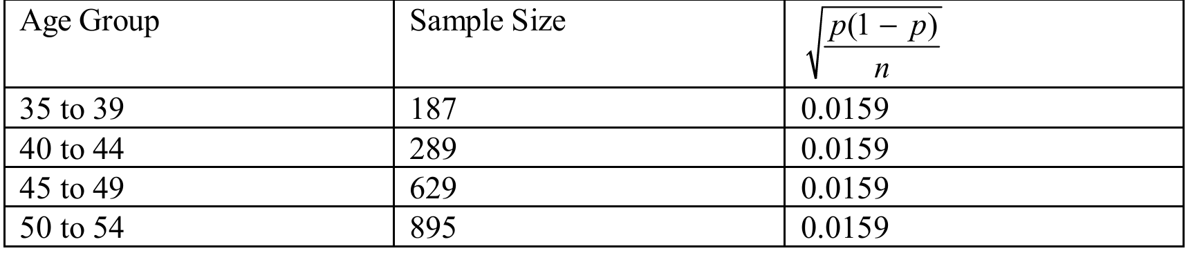
The total of all \(p(1-p)\) values is:
\( 0.0475 + 0.0736 + 0.1600 + 0.2275 = 0.5086 \)
Allocate the 2,000 subjects proportionally:
\( n_{35\text{-}39} = \frac{0.0475}{0.5086} \times 2000 = \boxed{186.79} \)
\( n_{40\text{-}44} = \frac{0.0736}{0.5086} \times 2000 = \boxed{289.42} \)
\( n_{45\text{-}49} = \frac{0.1600}{0.5086} \times 2000 = \boxed{629.18} \)
\( n_{50\text{-}54} = \frac{0.2275}{0.5086} \times 2000 = \boxed{894.61} \)
These four sample sizes sum to 2,000 and ensure that \(\sqrt{\dfrac{p(1-p)}{n}}\) is approximately equal across all four age-groups, producing confidence intervals of equal width.