AP Statistics 3.13 Carrying Out a Test for the Difference Between Two Population Proportions- Exam Style Questions - FRQs - New Syllabus

Question

A large exercise center has several thousand members from age $18$ to $55$ years and several thousand members age $56$ and older. The manager of the center is considering offering online fitness classes. The manager is investigating whether members’ opinions of taking online fitness classes differ by age.

The manager selected a random sample of $170$ exercise center members ages $18$ to $55$ years and a second random sample of $230$ exercise center members ages $56$ years and older. Each sampled member was asked whether they would be interested in taking online fitness classes. The manager found that $51$ of the $170$ sampled members ages $18$ to $55$ years and that $79$ of the $230$ sampled members ages $56$ years and older said they would be interested in taking online fitness classes.

At a significance level of $\alpha=0.05$, do the data provide convincing statistical evidence of a difference in the proportion of all exercise center members ages $18$ to $55$ years who would be interested in taking online fitness classes and the proportion of all exercise center members ages $56$ years and older who would be interested in taking online fitness classes? Complete the appropriate inference procedure to justify your response.

Most-appropriate topic codes (AP Statistics):

• Topic $3.12$ — Setting Up a Test for the Difference Between Two Population Proportions (Entire Question)
• Topic $3.13$ — Carrying Out a Test for the Difference Between Two Population Proportions (Entire Question)

▶️ Answer/Explanation

To determine if there’s a significant difference between the two age groups, we will perform a two-sample $z$-test for a difference in population proportions.

First, we need to state our hypotheses.
Let $p_{\text{younger}}$ represent the true proportion of members aged $18$ to $55$ who are interested in taking online fitness classes.
Let $p_{\text{older}}$ represent the true proportion of members aged $56$ and older who are interested in taking online fitness classes.
Null Hypothesis, $H_0: p_{\text{younger}} = p_{\text{older}}$
Alternative Hypothesis, $H_a: p_{\text{younger}} \neq p_{\text{older}}$

Next, we check the conditions:
1. Randomness: Both samples are stated as being randomly selected.
2. Independence ($10\%$ condition): The samples are drawn without replacement, but since $170 \times 10 = 1700$ and $230 \times 10 = 2300$ are both less than the “several thousand” members in each population, the condition is met.
3. Large Counts: The combined proportion is $\hat{p}_c = \dfrac{51 + 79}{170 + 230} = \dfrac{130}{400} = 0.325$.
The expected successes and failures are $170(0.325) = 55.25$, $170(1 – 0.325) = 114.75$, $230(0.325) = 74.75$, and $230(1 – 0.325) = 155.25$. All expected values are at least $10$, so the sampling distribution is approximately normal.

Now, let’s calculate the test statistic and $p$-value.
The sample proportions are $\hat{p}_{\text{younger}} = \dfrac{51}{170} = 0.30$ and $\hat{p}_{\text{older}} = \dfrac{79}{230} \approx 0.3435$.
The test statistic is:
$z = \dfrac{\hat{p}_{\text{younger}} – \hat{p}_{\text{older}}}{\sqrt{\hat{p}_c(1 – \hat{p}_c)\left(\dfrac{1}{n_{\text{younger}}} + \dfrac{1}{n_{\text{older}}}\right)}}$
$z = \dfrac{0.30 – 0.3435}{\sqrt{0.325(1 – 0.325)\left(\dfrac{1}{170} + \dfrac{1}{230}\right)}} \approx -0.91$
For a two-sided test, the $p$-value is $2 \times P(Z < -0.91) \approx 0.362$.

Finally, we state our conclusion:
Because our $p$-value of $0.362$ is much greater than $\alpha = 0.05$, we fail to reject the null hypothesis. We do not have convincing statistical evidence that there is a difference in the true proportions of younger and older members who are interested in taking online fitness classes.

Question

Tumbleweed, commonly found in the western United States, is the dried structure of certain plants that are blown by the wind. Kochia, a type of plant that turns into tumbleweed at the end of the summer, is a problem for farmers because it takes nutrients away from soil that would otherwise go to more beneficial plants. Scientists are concerned that kochia plants are becoming resistant to the most commonly used herbicide, glyphosate.

In $2014$, $19.7$ percent of $61$ randomly selected kochia plants were resistant to glyphosate. In $2017$, $38.5$ percent of $52$ randomly selected kochia plants were resistant to glyphosate.

Do the data provide convincing statistical evidence, at the level of $\alpha=0.05$, that there has been an increase in the proportion of all kochia plants that are resistant to glyphosate?

Most-appropriate topic codes (AP Statistics):

• Topic $3.12$ — Setting Up a Test for the Difference of Two Population Proportions (Entire Question)
• Topic $3.13$ — Carrying Out a Test for the Difference of Two Population Proportions (Entire Question)

▶️ Answer/Explanation

We need to perform a two-sample z-test for a difference in proportions. Let $p_{14}$ and $p_{17}$ be the true proportions of resistant kochia plants in $2014$ and $2017$, respectively.

Our hypotheses are $H_0: p_{17} – p_{14} = 0$ against the alternative $H_a: p_{17} – p_{14} > 0$.

Assuming the samples are independent and random, we calculate the pooled proportion as $\hat{p}_c = \dfrac{61(0.197) + 52(0.385)}{61+52} \approx 0.2835$.

Since the expected counts $61(0.2835)$, $61(1-0.2835)$, $52(0.2835)$, and $52(1-0.2835)$ are all comfortably greater than $10$, the normal condition is satisfied.

Next, we calculate the test statistic: $z = \dfrac{0.385 – 0.197}{\sqrt{0.2835(0.7165)\left(\frac{1}{61} + \frac{1}{52}\right)}} \approx 2.21$.

This gives us a p-value of roughly $0.0135$.

Because the p-value $0.0135$ is less than our significance level $\alpha = 0.05$, we reject $H_0$. There is convincing statistical evidence that the proportion of resistant kochia plants has increased from $2014$ to $2017$.

Question

A researcher conducted a medical study to investigate whether taking a low-dose aspirin reduces the chance of developing colon cancer. As part of the study, $1,000$ adult volunteers were randomly assigned to one of two groups. Half of the volunteers were assigned to the experimental group that took a low-dose aspirin each day, and the other half were assigned to the control group that took a placebo each day. At the end of six years, $15$ of the people who took the low-dose aspirin had developed colon cancer and $26$ of the people who took the placebo had developed colon cancer. At the significance level $\alpha=0.05$ do the data provide convincing statistical evidence that taking a low-dose aspirin each day would reduce the chance of developing colon cancer among all people similar to the volunteers?

Most-appropriate topic codes (AP Statistics):

• Topic $3.12$ — Setting Up a Test for the Difference Between Two Population Proportions
• Topic $3.13$ — Carrying Out a Test for the Difference Between Two Population Proportions

▶️ Answer/Explanation

We need to perform a two-sample $z$-test for the difference in population proportions.

Hypotheses:
Let $p_{asp}$ be the true probability of developing colon cancer for adults similar to the volunteers taking low-dose aspirin, and $p_{plac}$ be the probability for those taking a placebo.
$H_0: p_{asp} = p_{plac}$
$H_a: p_{asp} < p_{plac}$

Conditions:
Randomness: The problem states volunteers were randomly assigned to the two groups.
Large Counts: $n_{asp}\hat{p}_{asp} = 15$, $n_{asp}(1-\hat{p}_{asp}) = 485$, $n_{plac}\hat{p}_{plac} = 26$, $n_{plac}(1-\hat{p}_{plac}) = 474$. All observed numbers of successes and failures are $\ge 10$, so the sampling distribution is approximately normal.

Test Statistic and P-value:
$\hat{p}_{asp} = \dfrac{15}{500} = 0.030$
$\hat{p}_{plac} = \dfrac{26}{500} = 0.052$
The combined (pooled) proportion is $\hat{p}_c = \dfrac{15 + 26}{500 + 500} = \dfrac{41}{1000} = 0.041$.
$z = \dfrac{0.030 – 0.052}{\sqrt{0.041(1 – 0.041)\left(\dfrac{1}{500} + \dfrac{1}{500}\right)}} = \dfrac{-0.022}{0.0125} \approx -1.75$
$p\text{-value} = P(Z < -1.75) \approx 0.0401$

Conclusion:
Because the $p\text{-value}$ of $0.0401$ is less than the significance level $\alpha = 0.05$, we reject the null hypothesis $H_0$.
There is convincing statistical evidence that taking a low-dose aspirin each day would reduce the chance of developing colon cancer among people similar to the volunteers.

Question

Psychologists interested in the relationship between meditation and health conducted a study with a random sample of $28$ men who live in a large retirement community. Of the men in the sample, $11$ reported that they participate in daily meditation and $17$ reported that they do not participate in daily meditation.

The researchers wanted to perform a hypothesis test of

$H_0 : p_m – p_c = 0$
$H_a : p_m – p_c < 0,$

where $p_m$ is the proportion of men with high blood pressure among all the men in the retirement community who participate in daily meditation and $p_c$ is the proportion of men with high blood pressure among all the men in the retirement community who do not participate in daily meditation.

(a) If the study were to provide significant evidence against $H_0$ in favor of $H_a$, would it be reasonable for the psychologists to conclude that daily meditation causes a reduction in blood pressure for men in the retirement community? Explain why or why not.

The psychologists found that of the $11$ men in the study who participate in daily meditation, $0$ had high blood pressure. Of the $17$ men who do not participate in daily meditation, $8$ had high blood pressure.

(b) Let $\hat{p}_m$ represent the proportion of men with high blood pressure among those in a random sample of $11$ who meditate daily, and let $\hat{p}_c$ represent the proportion of men with high blood pressure among those in a random sample of $17$ who do not meditate daily. Why is it not reasonable to use a normal approximation for the sampling distribution of $\hat{p}_m – \hat{p}_c$?

Although a normal approximation cannot be used, it is possible to simulate the distribution of $\hat{p}_m – \hat{p}_c$. Under the assumption that the null hypothesis is true, $10{,}000$ values of $\hat{p}_m – \hat{p}_c$ were simulated. The histogram below shows the results of the simulation.

(c) Based on the results of the simulation, what can be concluded about the relationship between blood pressure and meditation among men in the retirement community?

Most-appropriate topic codes (AP Statistics):

• Topic $1.13$ — Experimental Design (Part $ \mathrm{a} $)
• Topic $3.12$ — Setting Up a Test for the Difference Between Two Population Proportions (Part $ \mathrm{b} $)
• Topic $3.13$ — Carrying Out a Test for the Difference Between Two Population Proportions (Part $ \mathrm{c} $)
• Topic $2.3$ — Estimating Probabilities Using Simulation (Part $ \mathrm{c} $)

▶️ Answer/Explanation

(a)

No, it would not be reasonable to conclude that daily meditation causes a reduction in blood pressure. This study is an observational study — the men themselves chose whether or not to meditate; no treatment was randomly assigned. Because there was no randomization of treatment, cause-and-effect conclusions cannot be drawn from the results. Men who choose to meditate may differ from men who don’t in other important ways that are also related to blood pressure, such as being more health-conscious, exercising more, or having lower stress in general. These potential confounding variables make it impossible to isolate meditation as the cause.

(b)

For a normal approximation to be valid for the sampling distribution of $\hat{p}_m – \hat{p}_c$, we need the number of successes and failures in each group to each be at least $10$. First, compute the combined sample proportion of successes:
$\hat{p} = \frac{0 + 8}{11 + 17} = \frac{8}{28} \approx 0.286$
Then check each group:
For the meditation group $(n_m = 11)$:
$n_m \hat{p} = 11 \times \frac{8}{28} \approx 3.14 < 10 \quad \text{(condition fails)}$
For the non-meditation group $(n_c = 17)$:
$n_c \hat{p} = 17 \times \frac{8}{28} \approx 4.86 < 10 \quad \text{(condition fails)}$
Since the expected number of successes in both groups is less than $10$, the normal approximation condition is not met, and it is not reasonable to use a normal approximation for the sampling distribution of $\hat{p}_m – \hat{p}_c$.

(c)

First, compute the observed value of the sample statistic from the data:
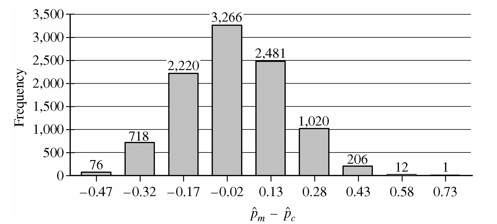
$\hat{p}_m – \hat{p}_c = \frac{0}{11} – \frac{8}{17} \approx -0.47$
From the simulation histogram, only $76$ out of $10{,}000$ simulated values were $-0.47$ or less (the most extreme negative outcome), giving an approximate $p$-value of:
$p\text{-value} \approx \frac{76}{10{,}000} = 0.0076$

Since this $p$-value of $0.0076$ is very small (less than any common significance level such as $\alpha = 0.05$), we reject $H_0$. There is convincing statistical evidence that men in this retirement community who meditate daily have a lower rate of high blood pressure than men who do not meditate. However, because this is an observational study, we can only conclude that meditation is associated with lower blood pressure — we cannot conclude that meditation causes a reduction in blood pressure.

Question

A survey organization conducted telephone interviews in December $2008$ in which $1,009$ randomly selected adults in the United States responded to the following question.

Of the $1,009$ adults surveyed, $676$ responded “yes.” In December $2007$, $622$ of $1,020$ randomly selected adults in the United States had responded “yes” to the same question. Do the data provide convincing evidence that the proportion of adults in the United States who would respond “yes” to the question changed from December $2007$ to December $2008$ ?

Most-appropriate topic codes (AP Statistics):

• Topic 3.12 — Setting Up a Test for the Difference Between Two Population Proportions (Entire Question)
• Topic 3.13 — Carrying Out a Test for the Difference Between Two Population Proportions (Entire Question)

▶️ Answer/Explanation

Step 1: Identify the parameters and state the hypotheses.

Let $p_{07}$ represent the true population proportion of all adults in the United States who would have answered “yes” in December 2007.
Let $p_{08}$ represent the true population proportion of all adults in the United States who would have answered “yes” in December 2008.
The hypotheses to be tested are:
$H_0: p_{07} = p_{08}$ (or $p_{07} – p_{08} = 0$)
$H_a: p_{07} \ne p_{08}$ (or $p_{07} – p_{08} \ne 0$)

Step 2: Identify the statistical test procedure and verify the inference conditions.

The appropriate procedure is a two-sample $z$-test for a difference between two population proportions.
Let’s check the necessary conditions:
1. Randomization Condition: The data must be collected via independent random sampling from the populations.
• Verification: This is satisfied because the problem specifies that the surveys involved “randomly selected adults” in both years.
2. Independence Condition (10% Rule): The sample sizes must be less than 10% of the entire populations when sampling without replacement.
• Verification: It is completely certain that 1,020 and 1,009 adults are both well under 10% of the hundreds of millions of adults living in the United States.
3. Large Counts / Normality Condition: The number of successes and failures in both samples must all be at least 10 to assume a normal sampling distribution.
• Sample 2007: $n_{07}\hat{p}_{07} = 622 \ge 10$ successes, and $n_{07}(1 – \hat{p}_{07}) = 1,020 – 622 = 398 \ge 10$ failures.
• Sample 2008: $n_{08}\hat{p}_{08} = 676 \ge 10$ successes, and $n_{08}(1 – \hat{p}_{08}) = 333 \ge 10$ failures.
Since all counts are much larger than 10, the normality condition is satisfied.

Step 3: Calculate the test statistic and the resulting $p$-value.
First, calculate the individual sample proportions:
$\hat{p}_{07} = \dfrac{622}{1,020} \approx 0.6098$
$\hat{p}_{08} = \dfrac{676}{1,009} \approx 0.6700$
Next, calculate the pooled proportion ($\hat{p}_c$) under the null hypothesis assumption that the two population parameters are identical:
$\hat{p}_c = \dfrac{\text{Total Successes}}{\text{Total Sample Size}} = \dfrac{622 + 676}{1,020 + 1,009} = \dfrac{1,298}{2,029} \approx 0.6397$
Now, calculate the standard error using the pooled proportion value:
$\text{SE} = \sqrt{\hat{p}_c(1 – \hat{p}_c)\left(\dfrac{1}{n_{07}} + \dfrac{1}{n_{08}}\right)} = \sqrt{(0.6397)(0.3603)\left(\dfrac{1}{1,020} + \dfrac{1}{1,009}\right)}$
$\text{SE} = \sqrt{(0.2305)(0.001971)} = \sqrt{0.0004543} \approx 0.02131$
Compute the standard $z$-test statistic:
$z = \dfrac{\hat{p}_{07} – \hat{p}_{08}}{\text{SE}} = \dfrac{0.6098 – 0.6700}{0.02131} = \dfrac{-0.0602}{0.02131} \approx -2.82$
Using a standard normal table for a two-tailed alternative hypothesis test ($H_a: \ne$):
$p\text{-value} = 2 \cdot P(Z \le -2.82) = 2 \cdot (0.0024) = 0.0048$

Step 4: Draw a conclusion in the context of the problem.

Because the obtained $p$-value of $0.0048$ is much smaller than any standard significance level like $\alpha = 0.05$, we reject the null hypothesis $H_0$.
There is very strong, convincing evidence that the true population proportion of adults in the United States who think television commercials are effective changed between December 2007 and December 2008 (specifically, the data suggests the proportion increased).

Question

A French study was conducted in the 1990s to compare the effectiveness of using an instrument called a cardiopump with the effectiveness of using traditional cardiopulmonary resuscitation (CPR) in saving lives of heart attack victims. Heart attack patients in participating cities were treated with either a cardiopump or CPR, depending on whether the individual’s heart attack occurred on an even-numbered or an odd-numbered day of the month. Before the start of the study, a coin was tossed to determine which treatment, a cardiopump or CPR, was given on the even-numbered days. The other treatment was given on the odd-numbered days. In total, 754 patients were treated with a cardiopump, and 37 survived at least one year; while 746 patients were treated with CPR, and 15 survived at least one year.

(a) The conditions for inference are satisfied in the study. State the conditions and indicate how they are satisfied.

(b) Perform a statistical test to determine whether the survival rate for patients treated with a cardiopump is significantly higher than the survival rate for patients treated with CPR.

Most-appropriate topic codes (AP Statistics):

• Topic $3.12$ — Setting Up a Test for the Difference Between Two Population Proportions (Part $\mathrm{b}$: hypotheses and test selection)
• Topic $3.13$ — Carrying Out a Test for the Difference Between Two Population Proportions (Part $\mathrm{b}$: test statistic, $p$-value, and conclusion)
• Topic $3.9$ — Sampling Distributions for the Difference Between Sample Proportions (Part $\mathrm{a}$: large counts condition for inference)
• Topic $1.13$ — Experimental Design (Part $\mathrm{a}$: random assignment of treatments)

▶️ Answer/Explanation

Let $p_A$ = true proportion of patients who survive at least one year if treated with the cardiopump.
Let $p_B$ = true proportion of patients who survive at least one year if treated with CPR.

(a)
The two conditions required for a two-sample $z$-test comparing proportions in an experiment are:
Condition 1 — Random assignment of treatments: Before the study began, a coin was tossed to determine which treatment was assigned to even-numbered days and which to odd-numbered days. This coin toss serves as a reasonable approximation to randomly assigning the two treatments to the available subjects, so this condition is satisfied.
Condition 2 — Sufficiently large sample sizes: All four counts (successes and failures for each group) must be at least 5. Checking:
$n_A \hat{p}_A = 37 \geq 5, \quad n_A(1-\hat{p}_A) = 754 – 37 = 717 \geq 5$
$n_B \hat{p}_B = 15 \geq 5, \quad n_B(1-\hat{p}_B) = 746 – 15 = 731 \geq 5$
All four values are well above 5, so the large sample condition is satisfied.

(b)

Step 1 — Hypotheses:
$H_0: p_A = p_B \quad \text{(or } p_A – p_B = 0\text{)}$
$H_a: p_A > p_B \quad \text{(or } p_A – p_B > 0\text{)}$

Step 2 — Test: Two-sample $z$-test for proportions (one-sided).

Step 3 — Compute the test statistic:
First, compute the pooled sample proportion:
$\hat{p} = \frac{n_A \hat{p}_A + n_B \hat{p}_B}{n_A + n_B} = \frac{37 + 15}{754 + 746} = \frac{52}{1500} \approx 0.0347$
Now compute the $z$-statistic:
$z = \frac{\hat{p}_A – \hat{p}_B}{\sqrt{\hat{p}(1-\hat{p})\left(\dfrac{1}{n_A} + \dfrac{1}{n_B}\right)}}$
$z = \frac{\dfrac{37}{754} – \dfrac{15}{746}}{\sqrt{(0.0347)(1 – 0.0347)\left(\dfrac{1}{754} + \dfrac{1}{746}\right)}} \approx 3.066$
The corresponding one-sided $p$-value is:
$p\text{-value} = P(Z > 3.066) \approx 0.0011$

Step 4 — Conclusion:
Since the $p$-value of $0.0011$ is much less than any reasonable significance level (such as $\alpha = 0.05$ or $\alpha = 0.01$), we reject $H_0$.
There is strong statistical evidence that the proportion of patients who survive at least one year is higher when treated with the cardiopump than when treated with CPR — that is, the cardiopump has a significantly higher survival rate than CPR.

Question

Researchers want to determine whether drivers are significantly more distracted while driving when using a cell phone than when talking to a passenger in the car. In a study involving 48 people, 24 people were randomly assigned to drive in a driving simulator while using a cell phone. The remaining 24 were assigned to drive in the driving simulator while talking to a passenger in the simulator. Part of the driving simulation for both groups involved asking drivers to exit the freeway at a particular exit. In the study, 7 of the 24 cell phone users missed the exit, while 2 of the 24 talking to a passenger missed the exit.

(a) Would this study be classified as an experiment or an observational study? Provide an explanation to support your answer.

(b) State the null and alternative hypotheses of interest to the researchers.

(c) One test of significance that you might consider using to answer the researchers’ question is a two-sample $z$-test. State the conditions required for this test to be appropriate. Then comment on whether each condition is met.

(d) Using an advanced statistical method for small samples to test the hypotheses in part (b), the researchers report a $p$-value of 0.0683. Interpret, in everyday language, what this $p$-value measures in the context of this study and state what conclusion should be made based on this $p$-value.

Most-appropriate topic codes (AP Statistics):

• Topic 1.13 — Experimental Design (Part $\mathrm{a}$)
• Topic 3.12 — Setting Up a Test for the Difference Between Two Population Proportions (Part $\mathrm{b}$)
• Topic 3.13 — Carrying Out a Test for the Difference Between Two Population Proportions (Part $\mathrm{c}$)
• Topic 3.6 — p-Values (Part $\mathrm{d}$)
• Topic 3.13 — Carrying Out a Test for the Difference Between Two Population Proportions (Part $\mathrm{d}$)

▶️ Answer/Explanation

(a)

This study is classified as an experiment, not an observational study.
The key reason is that the researchers actively imposed treatments on the subjects — they randomly assigned drivers to one of two conditions: driving while using a cell phone, or driving while talking to a passenger.
In an observational study, researchers simply observe subjects without intervening; here, the environment was deliberately controlled and manipulated, which is the defining feature of an experiment.
$\boxed{\text{Experiment — treatments (cell phone vs. passenger) were actively imposed on randomly assigned subjects.}}$

(b)

Let $p_{\text{cell}}$ = the population proportion of drivers who miss the exit while talking on a cell phone.
Let $p_{\text{pass}}$ = the population proportion of drivers who miss the exit while talking to a passenger.
$H_0: p_{\text{cell}} = p_{\text{pass}}$ (no difference in the proportion of drivers who miss the exit between the two groups)
$H_a: p_{\text{cell}} > p_{\text{pass}}$ (a greater proportion of cell phone users miss the exit compared to passenger talkers)
$\boxed{H_0: p_{\text{cell}} = p_{\text{pass}}, \quad H_a: p_{\text{cell}} > p_{\text{pass}}}$

(c)

The two conditions required for a two-sample $z$-test for proportions are:
Condition 1 — Independent random samples or random assignment: The problem states that the 48 participants were randomly assigned to the two groups, so this condition is met.
Condition 2 — Large sample sizes (each of $n_1\hat{p}_1$, $n_1(1-\hat{p}_1)$, $n_2\hat{p}_2$, $n_2(1-\hat{p}_2)$ must be $\geq 10$):
For the cell phone group: $n_1\hat{p}_1 = 24\cdot\dfrac{7}{24} = 7 < 10$
For the passenger group: $n_2\hat{p}_2 = 24\cdot\dfrac{2}{24} = 2 < 10$
Both groups fail the large sample condition, so this condition is not met. A two-sample $z$-test is therefore not appropriate for this situation.
$\boxed{\text{Condition 1 met (random assignment); Condition 2 NOT met } (n\hat{p} < 10 \text{ for both groups).}}$

(d)

In everyday language, the $p$-value of $0.0683$ means: assuming that cell phone use and talking to a passenger are equally distracting (i.e., $H_0$ is true), there is about a $6.83\%$ chance of observing a difference in missed-exit proportions as large as or larger than what was seen in this study just by random chance alone.
Since the $p$-value of $0.0683$ is greater than $\alpha = 0.05$, we fail to reject $H_0$. We do not have statistically significant evidence at the 5% level to conclude that drivers using a cell phone are more distracted (as measured by missing the freeway exit) than drivers talking to a passenger.
$\boxed{p\text{-value} = 0.0683 > 0.05 \Rightarrow \text{Fail to reject } H_0; \text{ insufficient evidence that cell phone use causes more distraction.}}$

Question

Scientists interested in preserving natural habitats and minimizing the possible extinction of certain bird species conducted a study to determine if it is better for conservation groups to purchase a few large nature preserves or many small preserves in order to meet these goals.

The scientists studied 13 randomly selected islands of different sizes to determine the risk of extinction for bird species. Islands are thought to be a good imitation of what would happen in a nature preserve because of their isolation. If a species lived on only one island, it was considered to be at risk. Scientists have determined that whether or not one species becomes extinct is independent of whether or not another species becomes extinct.

In 1990 scientists counted the number of at-risk species on each of the selected islands. They returned to each of these islands in the year 2000 to see whether the species still existed on the islands. Species that were present in 1990 but absent in 2000 were considered extinct. Data collected by the scientists are given in the table below.

(a) One scientist involved in the study believes that large islands (those with areas greater than 25 square kilometers) are more effective than small islands (those with areas of no more than 25 square kilometers) for protecting at-risk species. The scientist noted that for this study, a total of 19 of the 208 species on the large islands became extinct, whereas a total of 66 of the 299 species on the small islands became extinct. Assume that the probability of extinction is the same for all at-risk species on large islands and the same for all at-risk species on small islands. Do these data support the scientist’s belief? Give appropriate statistical justification for your answer.

(b) Another scientist who worked on this study thinks that the proportion of species that become extinct is more directly related to the size of the islands than simply to whether the islands are grouped as large or small. This scientist investigated the relationship between the proportion of extinct birds and the area, in square kilometers, of islands. A least squares analysis was conducted on the proportion extinct and $\ln(\text{area})$. The regression analysis output, the scatterplot, and the residual plot are shown below.

Estimate the slope of the least squares regression line using a 95 percent confidence interval. Interpret your answer in the context of this situation.

(c) In part (a), the scientist assumed that the probability of a species becoming extinct is the same for each of the large islands. Similarly, the scientist assumed that the probability is the same for each of the small islands. Based on your answer in part (b), do you think this is a reasonable assumption? Explain.

(d) A conservation group with a long-term goal of preserving species believes that all at-risk species will disappear whenever land inhabited by those species is developed. It has an opportunity to purchase land in an area about to be developed. The group has a choice of creating one large nature preserve with an area of 45 square kilometers and containing 70 at-risk species, or 5 small nature preserves, each with an area of 3 square kilometers and each containing 16 at-risk species unique to that preserve. Which choice would you recommend and why?

Most-appropriate topic codes (AP Statistics):

• Topic 3.12 — Setting Up a Test for the Difference Between Two Population Proportions (Part $\mathrm{a}$)
• Topic 3.13 — Carrying Out a Test for the Difference Between Two Population Proportions (Part $\mathrm{a}$)
• Topic 5.5 — Least-Squares Regression (Part $\mathrm{b}$)
• Topic 5.4 — Residuals (Part $\mathrm{c}$)
• Topic 5.5 — Least-Squares Regression (Part $\mathrm{d}$

▶️ Answer/Explanation

(a)
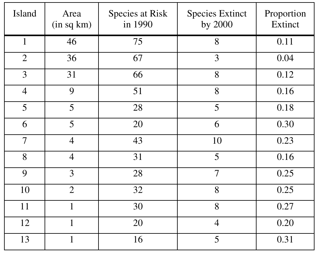
We want to test whether the proportion of species going extinct is smaller on large islands than on small islands. Let $p_L$ be the true proportion of at-risk species that become extinct on large islands, and $p_S$ be the true proportion on small islands.
The hypotheses are:
$H_0: p_L – p_S = 0$
$H_a: p_L – p_S < 0$
We use a two-sample $z$-test for the difference in proportions. The sample proportions are:
$\hat{p}_L = \frac{19}{208} \approx 0.091, \qquad \hat{p}_S = \frac{66}{299} \approx 0.221$
Check conditions — all expected counts must be at least 5:
$n_L\hat{p}_L = 19,\quad n_L(1-\hat{p}_L) = 189,\quad n_S\hat{p}_S = 66,\quad n_S(1-\hat{p}_S) = 233$
All values are well above 5, so we may proceed.
The pooled sample proportion is:
$\hat{p} = \frac{19+66}{208+299} = \frac{85}{507} \approx 0.168$
The test statistic is:
$z = \frac{\hat{p}_L – \hat{p}_S}{\sqrt{\hat{p}(1-\hat{p})\left(\dfrac{1}{n_L}+\dfrac{1}{n_S}\right)}} = \frac{0.091 – 0.221}{\sqrt{(0.168)(0.832)\left(\dfrac{1}{208}+\dfrac{1}{299}\right)}} = \frac{-0.130}{0.034} \approx -3.82$
The corresponding $p$-value $\approx 0.00006$, which is essentially $0$.
Since the $p$-value is far less than any reasonable significance level, we reject $H_0$. There is very strong statistical evidence that the proportion of species going extinct is smaller for large islands than for small islands, supporting the scientist’s belief.
$\boxed{z \approx -3.82, \quad p\text{-value} \approx 0.00006 \quad \Rightarrow \quad \text{Reject } H_0}$

(b)
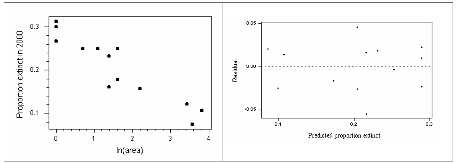
We construct a 95% confidence interval for the slope $\beta$ of the regression of proportion extinct on $\ln(\text{area})$.
From the regression output: $\hat{b} = -0.05323$, $SE_b = 0.00618$, and $df = n – 2 = 13 – 2 = 11$.
The critical value from the $t$-table with $df = 11$ at the 95% level is $t^* = 2.201$.
The confidence interval is:
$\hat{b} \pm t^* \cdot SE_b = -0.05323 \pm 2.201(0.00618)$
$-0.05323 \pm 0.01360$
$\boxed{(-0.0668,\ -0.0396)}$
We are 95% confident that for every 1-unit increase in $\ln(\text{area})$, the mean proportion of species going extinct decreases by somewhere between $0.0396$ and $0.0668$. In plain terms, larger islands are associated with a meaningfully lower extinction rate, and this relationship is statistically significant.

(c)
The assumption is not reasonable. The regression analysis in part (b) shows that the proportion of species going extinct decreases steadily as island area increases — it is a continuous relationship, not a step function that jumps only between “large” and “small” groups.
Within the large island group, areas ranged from 31 to 46 sq km, and within the small island group, areas ranged from 1 to 9 sq km — meaning extinction probabilities varied considerably within each group as well.
Because extinction probability depends on actual area and not just on a binary large/small classification, the assumption that all large islands share one common extinction probability and all small islands share another is not supported by the data.

(d)
We use the regression model $\widehat{\text{prop extinct}} = 0.28996 – 0.05323\ln(\text{area})$ to estimate extinction proportions for each option.
Option 1 — One large preserve (area = 45 sq km, 70 species):
$\widehat{\text{prop extinct}} = 0.28996 – 0.05323\ln(45) = 0.28996 – 0.05323(3.807) \approx 0.28996 – 0.20261 \approx 0.0873$
Expected extinctions: $70 \times 0.0873 \approx 6.1$ species
Expected survivors: $70 – 6.1 \approx \mathbf{63.9 \approx 64}$ species

Option 2 — Five small preserves (each area = 3 sq km, 16 species each; 80 total):
$\widehat{\text{prop extinct}} = 0.28996 – 0.05323\ln(3) = 0.28996 – 0.05323(1.099) \approx 0.28996 – 0.05850 \approx 0.2315$
Expected extinctions per preserve: $16 \times 0.2315 \approx 3.7$ species
Total expected extinctions: $5 \times 3.7 \approx 18.5$ species
Expected survivors: $80 – 18.5 \approx \mathbf{61.5 \approx 62}$ species

The one large preserve is expected to save approximately 64 species, compared to about 62 species across the five small preserves. We recommend creating one large nature preserve, as it leads to a greater expected number of surviving species, and larger areas have been shown to have substantially lower extinction rates per species.
$\boxed{\text{Recommend: One large preserve (45 sq km)} \Rightarrow \approx 64 \text{ species saved vs. } \approx 62 \text{ for five small preserves}}$

Question

In order to monitor the populations of birds of a particular species on two islands, the following procedure was implemented.

Researchers captured an initial sample of 200 birds of the species on Island A; they attached leg bands to each of the birds, and then released the birds. Similarly, a sample of 250 birds of the same species on Island B was captured, banded, and released. Sufficient time was allowed for the birds to return to their normal routine and location.

Subsequent samples of birds of the species of interest were then taken from each island. The number of birds captured and the number of birds with leg bands were recorded. The results are summarized in the following table.

Assume that both the initial sample and the subsequent samples that were taken on each island can be regarded as random samples from the population of birds of this species.

(a) Do the data from the subsequent samples indicate that there is a difference in proportions of the banded birds on these two islands? Give statistical evidence to support your answer.

(b) Researchers can estimate the total number of birds of this species on an island by using information on the number of birds in the initial sample and the proportion of banded birds in the subsequent sample. Use this information to estimate the total number of birds of this species on Island A. Show your work.

(c) The analyses in parts (a) and (b) assume that the samples of birds captured in both the initial and subsequent samples can be regarded as random samples of the population of birds of this species that live on the respective islands. This is a common assumption made by wildlife researchers. Describe two concerns that should be addressed before making this assumption.

Most-appropriate topic codes (AP Statistics):

• Topic 3.12 — Setting Up a Test for the Difference Between Two Population Proportions (Part a)
• Topic 3.13 — Carrying Out a Test for the Difference Between Two Population Proportions (Part a)
• Topic 3.1 — Estimators (Part b)
• Topic 1.11 — Random Sampling (Part c)
• Topic 1.12 — Potential Problems with Sampling (Part c)

▶️ Answer/Explanation

(a)

Step 1: State hypotheses.
Let $p_A$ = true proportion of banded birds on Island A, and $p_B$ = true proportion of banded birds on Island B.
$H_0: p_A – p_B = 0 \qquad H_a: p_A – p_B \neq 0$
Step 2: Identify the test and check assumptions.
We use a two-sample $z$-test for a difference in proportions. The test statistic is:
$z = \dfrac{\hat{p}_A – \hat{p}_B}{\sqrt{\hat{p}(1-\hat{p})\left(\dfrac{1}{n_1} + \dfrac{1}{n_2}\right)}}$
The problem states the samples are random. Since the two islands are separate, the samples are independent. We check the large sample condition using the pooled estimate:
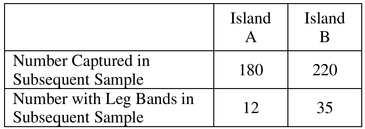
$\hat{p} = \dfrac{n_A\hat{p}_A + n_B\hat{p}_B}{n_A + n_B} = \dfrac{12 + 35}{180 + 220} = \dfrac{47}{400} = 0.1175$
Expected counts: $n_A\hat{p} = 21.15,\quad n_A(1-\hat{p}) = 158.85,\quad n_B\hat{p} = 25.85,\quad n_B(1-\hat{p}) = 194.15$
All expected counts are well above 5, so the large sample condition is satisfied.
Step 3: Compute the test statistic and p-value.
$\hat{p}_A = \dfrac{12}{180} = 0.067 \qquad \hat{p}_B = \dfrac{35}{220} = 0.159$
$z = \dfrac{0.067 – 0.159}{\sqrt{\dfrac{(0.1175)(0.8825)}{180} + \dfrac{(0.1175)(0.8825)}{220}}} = \dfrac{-0.092}{\sqrt{0.00105}} = \dfrac{-0.092}{0.032} = -2.875$
$\text{p-value} = 2 \times P(Z < -2.875) \approx 0.00429$
Step 4: State conclusion in context.
Since the p-value of $0.00429$ is less than $\alpha = 0.05$, we reject the null hypothesis. There is convincing statistical evidence that the proportions of banded birds on the two islands are different — Island B has a notably higher proportion of banded birds than Island A.

(b)

We use the capture-recapture logic: the proportion of banded birds in the subsequent sample estimates the proportion of banded birds in the whole population.
For Island A, the number of birds banded in the initial sample is $n_I = 200$, and the proportion of banded birds observed in the subsequent sample is:
$\hat{p}_S = \dfrac{12}{180} \approx 0.06667$
Setting this equal to the fraction of banded birds in the population:
$\hat{p}_S \approx \dfrac{n_I}{\text{population size}}$
Solving for the estimated population size:
$\text{Estimated population size} = \dfrac{n_I}{\hat{p}_S} = \dfrac{200}{12/180} = \dfrac{200 \times 180}{12} = \dfrac{36{,}000}{12} = \boxed{3{,}000 \text{ birds}}$

(c)

Two concerns that should be addressed before assuming the captures can be treated as random samples are:
Concern 1 — Differential catchability: Some birds may be more likely to be captured than others — for example, slower, older, or less wary birds might be caught at a higher rate than the general population. If the same birds that were easy to capture in the initial sample are also more likely to appear in the subsequent sample, then banded birds would be overrepresented in the subsequent sample, leading us to underestimate the true population size.
Concern 2 — Behavioural change after banding: Birds that were captured and banded in the initial sample may become more trap-shy (avoiding capture in the future) or, conversely, may be more conspicuous to predators due to the bands, altering their survival or behaviour. If banded birds are less likely to be recaptured, we would overestimate the population size. In either case, if banding changes the birds’ behaviour or survival, the subsequent sample can no longer be treated as a true random sample of the population.

Question

A study was conducted to determine if taking vitamin C reduces the occurrence of the flu. The study was conducted using 808 student volunteers who did not take a flu shot. The subjects were randomly assigned to one of two groups: a treatment group who received 1,000 milligrams of vitamin C daily or a control group who received a placebo flavored to taste like the vitamin C treatment. All participants were monitored to ensure that they adhered to their assigned treatment on a daily basis throughout the period of the study. At the end of the flu season, each subject’s medical record was reviewed by a physician to determine whether he or she had contracted the flu during the period of the study. The physician did not know which treatment each subject received. The results of the study are shown in the table below.

(a) Is this study an experiment or an observational study? Explain your answer.

(b) Based on this study, a health expert claims that there is evidence to suggest that vitamin C reduces the occurrence of the flu in the population of students who would volunteer for such a study. State the name of a test and the null and alternative hypotheses that the health expert could have used to support this claim. Do not carry out the test.

Most-appropriate topic codes (AP Statistics):

• Topic 1.13 — Experimental Design (Part a)
• Topic 3.12 — Setting Up a Test for the Difference Between Two Population Proportions (Part b)
• Topic 3.13 — Carrying Out a Test for the Difference Between Two Population Proportions (Part b)
• Topic 3.9 — Sampling Distributions for the Difference Between Sample Proportions (Part b)

▶️ Answer/Explanation

(a)

This study is an experiment, not an observational study.
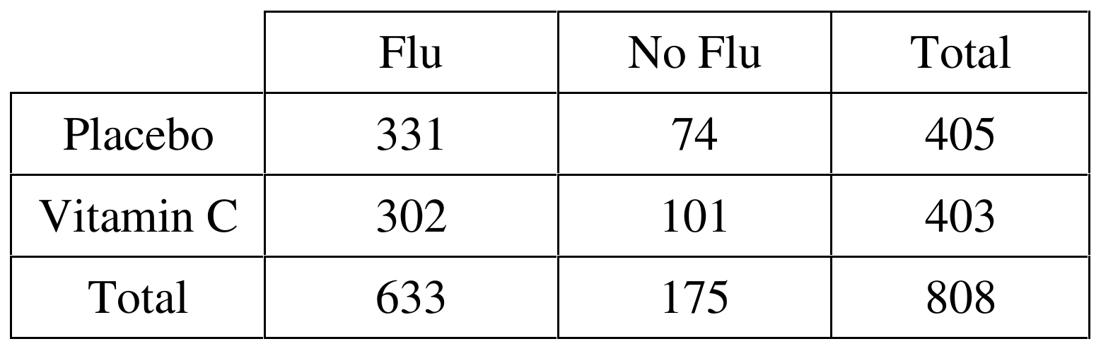
In an experiment, the researchers deliberately impose a treatment on the subjects — here, the researchers assigned subjects to either the vitamin C group or the placebo group, rather than simply observing what subjects naturally chose to do.
Crucially, subjects were randomly assigned to the two treatment groups, which is the hallmark of a well-designed experiment and allows for causal conclusions to be drawn.
The use of a placebo and blind evaluation by a physician further strengthen this as a controlled experiment.

(b)

The health expert could use a two-proportion $z$-test to support this claim.
Let $p_T$ be the true proportion of students (in the population of volunteers) who contract the flu when taking vitamin C, and let $p_C$ be the true proportion who contract the flu when taking a placebo.
The hypotheses are:
$ H_0: p_T – p_C = 0 \quad \text{(vitamin C has no effect on flu occurrence)} $
$ H_a: p_T – p_C < 0 \quad \text{(vitamin C reduces flu occurrence)} $
Equivalently, this can be written as $H_0: p_T = p_C$ versus $H_a: p_T < p_C$, where a one-sided alternative is used because the claim is specifically that vitamin C reduces the occurrence of flu.

AP Statistics 3.13 Carrying Out a Test for the Difference Between Two Population Proportions- Exam Style Questions - FRQs - New Syllabus

Question

Question

Question

Question

Question

Question

Question

Question

Question

Question

Resources

Members

Company