Home / AP® Exam / AP® Statistics / AP Statistics 3.15 Carrying Out a Chi-Square Test for Homogeneity or Independence- Exam Style Questions – MCQs

AP Statistics 3.15 Carrying Out a Chi-Square Test for Homogeneity or Independence- Exam Style Questions - MCQs - New Syllabus

Question 

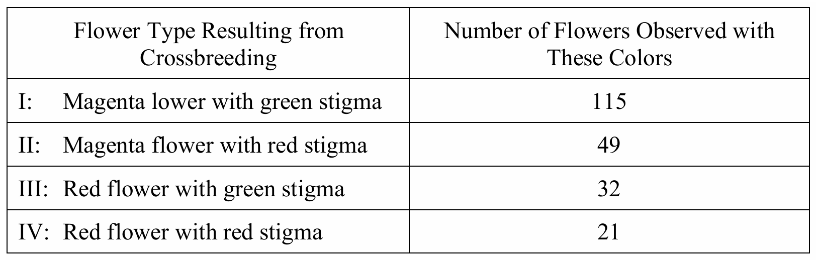
In an experiment, two different species of flowers were crossbred. The resulting flowers from this crossbreeding experiment were classified, by color of flower and stigma, into one of four groups, as shown in the table below.

A biologist expected that the ratio of 9:3:3:1 for the flower types I:II:III:IV, respectively, would result from this crossbreeding experiment. From the data above, a value of approximately 8.04 was computed for the chi-square test statistic. Are the observed results inconsistent with the expected ratio at the 5 percent level of significance?

(A) Yes, because the computed value is greater than the critical value.
(B) Yes, because the computed value is less than the critical value.
(C) No, because the computed value is less than the critical value.
(D) No, because the computed value is greater than the critical value.
(E) It cannot be determined because some of the expected counts are not large enough to use the test.

▶️ Answer/Explanation

This is a chi-square goodness-of-fit test with four categories, so the degrees of freedom are:
\( df = 4 – 1 = 3 \)
At the 5% significance level, the critical value is:
\( \chi^2_{0.05,3} \approx 7.815 \)
The computed test statistic is:
\( \chi^2 = 8.04 \)
Since:
\( 8.04 > 7.815 \)
we reject the null hypothesis and conclude that the observed results are inconsistent with the expected 9:3:3:1 ratio at the 5% significance level.

Answer: (A)

Question 

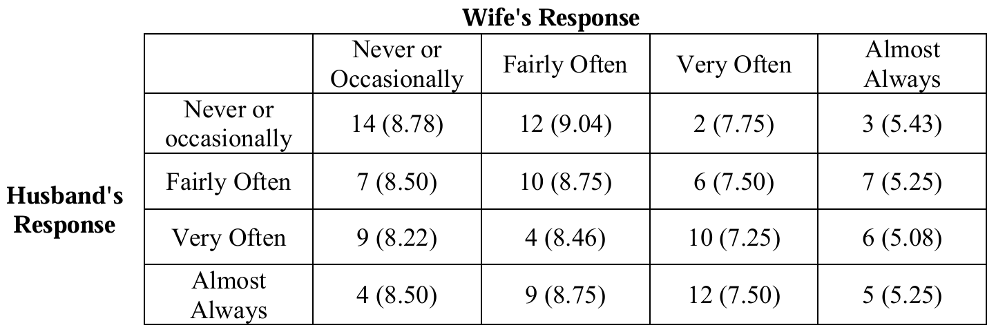
A survey of 120 randomly selected married couples asked each partner to rate how often they dine out as a couple. The results are presented below with expected counts in parentheses.

In testing to see if there is evidence of an association between the ratings of husbands and wives, a chi-square test statistic of 19.48 was calculated. Which of the following statements is correct?

(A) The data prove the couples’ ratings are associated.
(B) The data prove the couples’ ratings are not associated.
(C) There is sufficient evidence to suggest the couples’ ratings are associated at the 5% significance level but not at the 1% significance level.
(D) There is sufficient evidence to suggest the couples’ ratings are associated at the 1% significance level.
(E) The chi-square test should not have been used because four of the observed counts are less than 5.

▶️ Answer/Explanation
This is a chi-square test of independence. The degrees of freedom are:
\(df=(r-1)(c-1)\)
\(df=(4-1)(4-1)\)
\(df=9\)
The test statistic is:
\(\chi^2=19.48\)
For (df=9):
\(\chi^2_{0.05}=16.919\)
\(\chi^2_{0.01}=21.666\)
Since \(19.48 > 16.919\) the null hypothesis of independence is rejected at the 5% significance level.
However, \(19.48 < 21.666\) so the null hypothesis is not rejected at the 1% significance level.
Also, chi-square conditions are based on expected counts, not observed counts.
All expected counts shown are greater than 5, so the chi-square procedure is appropriate.
Therefore, there is sufficient evidence of an association at the 5% level but not at the 1% level.
Answer: (C)

Question 

To investigate the relationship between age and preference for two mayoral candidates in an upcoming election, a random sample of city residents was surveyed. The residents were asked which candidate they preferred, and each resident was classified into one of three age-groups. The test statistic for the appropriate hypothesis test was 3.7408. Approximately what is the probability that the observed responses would be as far or farther from the expected responses if there is no association between age-group and preference?

(A) 0.0001
(B) 0.1541
(C) 0.2908
(D) 0.5873
(E) 0.7117

▶️ Answer/Explanation

This is a chi-square test of independence because two categorical variables are being compared: age-group and candidate preference.

The table would have:

\(r=3\) age groups
\(c=2\) candidate preferences

Degrees of freedom:

\(df=(r-1)(c-1)\)
\(=(3-1)(2-1)\)
\(=2\)

Given the test statistic:

\(\chi^2=3.7408\)

Using a chi-square distribution with \(df=2\), the upper-tail probability is approximately:

\(P(\chi^2 \ge 3.7408)\approx 0.1541\)

This probability is the p-value, which represents the chance of observing results at least this extreme if there is truly no association between age-group and candidate preference.

Answer: (B)

Scroll to Top