
AP Statistics 3.2 Sampling Distributions for Sample Proportions- Exam Style Questions - FRQs - New Syllabus
Question

Most-appropriate topic codes (AP Statistics):
• Topic \(3.3\) — Constructing a Confidence Interval for a Population Proportion (Parts \( \mathrm{a} \), \( \mathrm{b} \))
• Topic \(3.4\) — Justifying a Claim Based on a Confidence Interval for a Population Proportion (Part \( \mathrm{a} \))
• Topic \(3.10\) — Constructing a Confidence Interval for the Difference Between Two Population Proportions (Part \( \mathrm{c} \))
▶️ Answer/Explanation
(a)
The appropriate procedure is a one-sample \(z\)-interval for a population proportion.
Let \(p\) = the true proportion of all adults in the United States who would have chosen the economy statement.
From the sample: \(\hat{p} = 0.37\), \(n = 1{,}048\), and the critical value for 95% confidence is \(z^* = 1.96\).
The confidence interval formula is:
\( \hat{p} \pm z^* \sqrt{\dfrac{\hat{p}(1-\hat{p})}{n}} \)
Substituting the values:
\( 0.37 \pm 1.96\sqrt{\dfrac{(0.37)(0.63)}{1{,}048}} \)
\( 0.37 \pm 1.96\sqrt{0.000222} \)
\( 0.37 \pm 1.96(0.0149) \)
\( 0.37 \pm 0.03 = (0.34,\ 0.40) \)
Interpretation: We are 95 percent confident that the interval from 0.34 to 0.40 captures the true proportion of all adults in the United States who would have chosen the economy statement.
(b)
This condition is necessary because the confidence interval formula for a population proportion relies on approximating the binomial distribution with a normal distribution. This approximation causes the sampling distribution of \(\hat{p}\) to be approximately normal, which is what allows us to use the \(z\)-critical value and construct a valid interval.
However, the normal approximation to the binomial works well only when both \(n\hat{p}\) and \(n(1-\hat{p})\) are at least 10. If either of these quantities is too small, the sampling distribution of \(\hat{p}\) will be noticeably skewed rather than approximately normal, and the confidence interval will not be reliable.
(c)
No, the two-sample \(z\)-interval for a difference between proportions is not an appropriate procedure here.
A key requirement for the two-sample \(z\)-interval is that the two proportions come from two independent samples. In this study, however, both proportions — the proportion choosing the environment statement and the proportion choosing the economy statement — come from the same single sample of 1,048 adults. Because each person was forced to choose between the two statements (or express no preference), the two proportions are not independent: knowing one proportion directly constrains the other. Since the independence condition is violated, the two-sample \(z\)-interval is not appropriate for this situation.
Question
Most-appropriate topic codes (AP Statistics):
• Topic \(3.4\) — Justifying a Claim Based on a Confidence Interval for a Population Proportion (Part \(\mathrm{a}\))
• Topic \(3.2\) — Sampling Distributions for Sample Proportions (Part \(\mathrm{b}\))
▶️ Answer/Explanation
(a)
Procedure: One-sample \(z\)-interval for a population proportion.
Conditions:
Random: The problem states the 50 songs were randomly selected. ✓
Large Counts: \(n\hat{p} = 50 \times 0.26 = 13 \geq 10\) and \(n(1-\hat{p}) = 50 \times 0.74 = 37 \geq 10\). ✓
Both conditions are satisfied, so we may proceed.
Calculation:
The sample proportion is:
\(\hat{p} = \frac{13}{50} = 0.26\)
For a 90% confidence interval, the critical value is \(z^* = 1.645\). The margin of error is:
\(ME = z^* \sqrt{\frac{\hat{p}(1-\hat{p})}{n}} = 1.645 \times \sqrt{\frac{0.26 \times 0.74}{50}}\)
\(ME = 1.645 \times \sqrt{\frac{0.1924}{50}} = 1.645 \times \sqrt{0.003848} = 1.645 \times 0.06203 \approx 0.102\)
The 90% confidence interval is:
\(\hat{p} \pm ME = 0.26 \pm 0.102 = \boxed{(0.158,\ 0.362)}\)
Interpretation: We are 90% confident that the true proportion of all songs on the digital music player that were loaded by Lori is between 0.158 and 0.362.
In plain terms — if we repeated this process many times, about 90% of the confidence intervals we’d construct would capture the actual fraction of songs that Lori loaded. Based on this one interval, our best guess is somewhere between roughly 16% and 36%.
(b)
The distinction between sampling with replacement and without replacement only matters meaningfully when the sample size is large relative to the population size. Here we check the ratio:
\(\frac{\text{Population size}}{\text{Sample size}} = \frac{2384}{50} = 47.7\)
Since the population is about 47.7 times larger than the sample, the sample of 50 represents only:
\(\frac{50}{2384} \approx 2.1\%\text{ of the population}\)
This is well below the standard 10% threshold. When the sample is this small relative to the population, removing a song from the pool (sampling without replacement) barely changes the probability of selecting any remaining song. For example:
Probability of selecting a specific song with replacement: \(\dfrac{1}{2384} \approx 4.195 \times 10^{-4}\)
Probability of selecting a specific song without replacement (after one song removed): \(\dfrac{1}{2383} \approx 4.196 \times 10^{-4}\)
The difference is negligible — on the order of \(10^{-7}\). Because the population is so large relative to the sample, the two sampling methods produce virtually identical results, and the confidence interval from part (a) is valid regardless of which method the player uses.
Question
Most-appropriate topic codes (AP Statistics):
• Topic 3.2 — Sampling Distributions for Sample Proportions (Part \(\mathrm{b}\))
• Topic 2.10 — The Binomial Distribution (Part \(\mathrm{c}\))
• Topic 3.6 — p-Values (Part \(\mathrm{d}\))
• Topic 3.7 — Carrying Out a Test for a Population Proportion (Part \(\mathrm{e}\))
• Topic 1.13 — Experimental Design (Part \(\mathrm{f}\))
▶️ Answer/Explanation
(a)
Let \(p\) be the population proportion of consumers who prefer Citrus Fresh. The hypotheses are:
\(H_0: p = 0.5\)
\(H_a: p \neq 0.5\)
A two-sided alternative is appropriate because Sunshine Farms wants to detect any difference in preference, not just preference for one particular juice.
(b)
The conditions for a one-proportion \(z\)-test require that both \(np\) and \(n(1-p)\) be at least 5 (or 10). Here:
\(np = 8 \times 0.5 = 4 < 5\)
\(n(1-p) = 8 \times 0.5 = 4 < 5\)
Since both values are less than 5, the large-sample normal approximation is not valid, and using a one-proportion \(z\)-test would not be appropriate for a sample of only \(n = 8\).
(c)
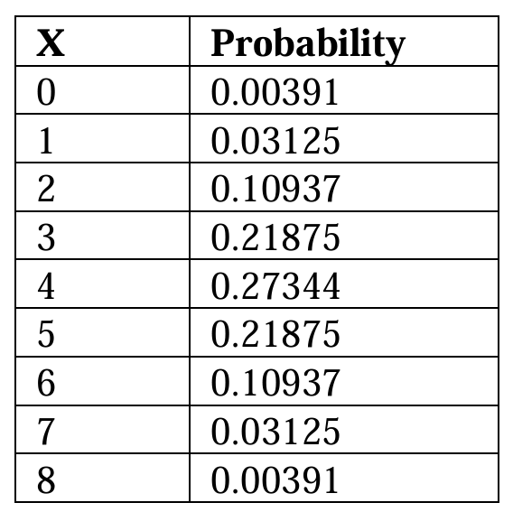
Under \(H_0\), \(X \sim \text{Binomial}(n = 8,\ p = 0.5)\). The probabilities are computed using:
\(P(X = x) = \binom{8}{x}(0.5)^x(0.5)^{8-x} = \binom{8}{x}(0.5)^8\)
(d)
No, it is not possible for the significance level to be exactly 0.05. Because \(X\) is a discrete random variable, the tail probabilities can only take specific values — there is no rejection region that gives a type I error probability of exactly 0.05.
The most extreme rejection region \((X = 0 \text{ or } X = 8)\) gives:
\(\alpha = 2 \times 0.00391 = 0.00782 < 0.05\)
The next possible rejection region \((X \leq 1 \text{ or } X \geq 7)\) gives:
\(\alpha = 2 \times (0.00391 + 0.03125) = 2 \times 0.03516 = 0.07031 > 0.05\)
Since no rejection region produces a type I error probability of exactly 0.05, a significance level of exactly 0.05 is not achievable with this test.
\(\boxed{\alpha = 0.05 \text{ is not achievable — the achievable levels jump from } 0.00782 \text{ to } 0.07031}\)
(e)
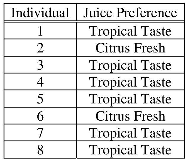
From the data, 2 out of 8 consumers preferred Citrus Fresh, so \(X = 2\).
Since this is a two-sided test, the \(p\)-value is the probability of observing a result at least as extreme as \(X = 2\) in either tail:
\(p\text{-value} = P(X \leq 2) + P(X \geq 6)\)
\(= 2 \times [P(X=0) + P(X=1) + P(X=2)]\)
\(= 2 \times (0.00391 + 0.03125 + 0.10937)\)
\(= 2 \times 0.14453 = 0.28906\)
Since the \(p\)-value of \(0.289\) is much larger than any reasonable significance level (e.g., \(\alpha = 0.05\) or \(\alpha = 0.07031\)), we fail to reject \(H_0\). There is not statistically significant evidence of a consumer preference between Citrus Fresh and Tropical Taste.
\(\boxed{p\text{-value} \approx 0.289 \implies \text{Fail to reject } H_0; \text{ no significant consumer preference detected}}\)
(f)
The most important recommendation is to increase the number of consumers in the study. With only \(n = 8\) consumers, the test has very low power — even a large true difference in preference (like 75% vs. 25%) may not produce a statistically significant result. Increasing the sample size would reduce the standard error of the estimated proportion \(\hat{p}\), making it easier to detect a real difference, and would allow the use of the large-sample one-proportion \(z\)-test since \(np \geq 5\) and \(n(1-p) \geq 5\) would be satisfied. For example, with \(n = 80\) and \(X = 20\) (same sample proportion of 0.25), the \(z\)-statistic would be approximately:
\(z = \frac{0.25 – 0.5}{\sqrt{\frac{0.5(0.5)}{80}}} \approx -4.47\)
which gives a \(p\)-value near zero, allowing a clear conclusion to be reached.
\(\boxed{\text{Recommendation: Increase sample size to increase power and enable use of the } z\text{-test}}\)
Question

Most-appropriate topic codes (AP Statistics):
• Topic 3.4 — Justifying a Claim Based on a Confidence Interval for a Population Proportion (Part a)
• Topic 3.1 — Estimators (Part b)
• Topic 3.2 — Sampling Distributions for Sample Proportions (Parts b, c)
▶️ Answer/Explanation
(a)
Procedure and Conditions:
We use a one-sample \(z\)-confidence interval for a proportion: \(\hat{p} \pm z^* \sqrt{\dfrac{\hat{p}(1-\hat{p})}{n}}\).
From the table, the sample of females in the 40–44 age-group has \(n = 370\). With 10% contracting the illness, \(\hat{p} = 0.10\).
Check conditions: The sample is a random sample from the HMO population. The expected number of successes is \(n\hat{p} = 370(0.10) = 37 > 5\) and the expected number of failures is \(n(1-\hat{p}) = 370(0.90) = 333 > 5\), so the sample size is large enough to proceed.
Mechanics:
\( \hat{p} \pm z^* \sqrt{\frac{\hat{p}(1-\hat{p})}{n}} = 0.10 \pm 1.96\sqrt{\frac{(0.10)(0.90)}{370}} \)
\( = 0.10 \pm 1.96\sqrt{\frac{0.09}{370}} = 0.10 \pm 1.96(0.01559) = 0.10 \pm 0.0306 \)
\( \boxed{(0.06943,\ 0.13057)} \)
Interpretation of the confidence interval:
We are 95% confident that the true proportion of the HMO’s 40–44 year old female patients who would contract this illness is between approximately 0.069 and 0.131 (i.e., between about 6.9% and 13.1%).
Interpretation of the 95% confidence level:
If we were to take many random samples of size 370 from this population and compute a 95% confidence interval from each sample, approximately 95% of those intervals would capture the true population proportion of 40–44 year old female HMO patients who contract the illness. In other words, the method we used to construct this interval will fail to contain the true proportion only about 5% of the time in repeated sampling.
(b)
The width of a confidence interval for a proportion is determined by the margin of error \(z^*\sqrt{\dfrac{\hat{p}(1-\hat{p})}{n}}\), which depends on both \(\hat{p}\) and \(n\).
When the sample proportions are equal (both 0.10), the only factor causing different interval widths is the different sample sizes — females had \(n = 370\) while males had \(n = 230\) in the 40–44 group, producing a wider interval for males.
To make the confidence interval widths equal for all 8 groups when sample proportions are equal, the sample sizes for all 8 groups must be equal.
With 2,000 total subjects and 8 groups, each group should receive a sample of size:
\( n = \frac{2000}{8} = \boxed{250 \text{ subjects per group}} \)
Equal sample sizes guarantee equal standard errors (and therefore equal interval widths) whenever the sample proportions are the same.
(c)
When sample proportions differ across groups, equal widths require not equal sample sizes but rather sample sizes proportional to \(\hat{p}(1-\hat{p})\) for each group — this keeps the standard error \(\sqrt{\dfrac{\hat{p}(1-\hat{p})}{n}}\) the same across all groups.
Compute \(p(1-p)\) for each age-group using the anticipated proportions: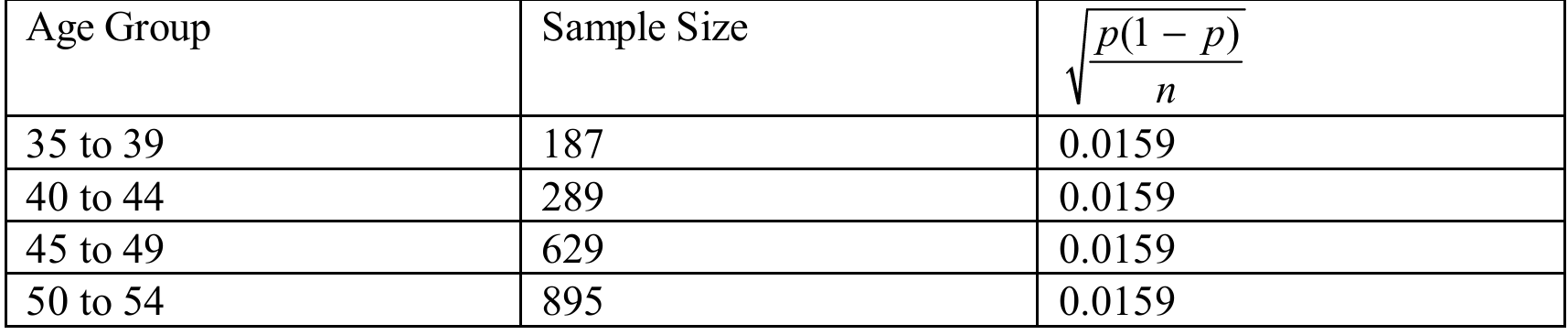
The total of all \(p(1-p)\) values is:
\( 0.0475 + 0.0736 + 0.1600 + 0.2275 = 0.5086 \)
Allocate the 2,000 subjects proportionally:
\( n_{35\text{-}39} = \frac{0.0475}{0.5086} \times 2000 = \boxed{186.79} \)
\( n_{40\text{-}44} = \frac{0.0736}{0.5086} \times 2000 = \boxed{289.42} \)
\( n_{45\text{-}49} = \frac{0.1600}{0.5086} \times 2000 = \boxed{629.18} \)
\( n_{50\text{-}54} = \frac{0.2275}{0.5086} \times 2000 = \boxed{894.61} \)
These four sample sizes sum to 2,000 and ensure that \(\sqrt{\dfrac{p(1-p)}{n}}\) is approximately equal across all four age-groups, producing confidence intervals of equal width.