
AP Statistics 3.3 Constructing a Confidence Interval for a Population Proportion- Exam Style Questions - FRQs - New Syllabus
Question
Most-appropriate topic codes (AP Statistics):
• Topic \(3.4\) — Justifying a Claim Based on a Confidence Interval for a Population Proportion (Part \( \mathrm{b} \))
▶️ Answer/Explanation
(a)
State: We will construct a one-sample z-interval for $p$, the true proportion of all teenagers in the United States who would respond that they use a video streaming service every day.
Plan:
• Random condition: The problem states that the data came from a “random sample.”
• 10% condition: $n = 920$, which is less than 10% of all teenagers in the United States.
• Large counts condition: The number of successes is $920(0.59) = 542.8 \ge 10$ and the number of failures is $920(0.41) = 377.2 \ge 10$. Both are at least 10, so the sampling distribution of $\hat{p}$ is approximately normal.
Do: The formula for the confidence interval is:
$ \hat{p} \pm z^* \sqrt{\frac{\hat{p}(1-\hat{p})}{n}} $
For a 95% confidence level, the critical value is $z^* = 1.96$. Substituting the values:
$ 0.59 \pm 1.96 \sqrt{\frac{0.59(0.41)}{920}} $
$ 0.59 \pm 1.96(0.0162) $
$ 0.59 \pm 0.0318 $
The 95% confidence interval is $(0.558, 0.622)$.
Conclude: We are 95% confident that the interval from 0.558 to 0.622 captures the true proportion of all teenagers in the United States who would respond that they use a video streaming service every day.
(b)
Yes, the sample data provide convincing statistical evidence that the true proportion is not 0.5.
Justification: The value 0.5 is not contained within the 95% confidence interval of $(0.558, 0.622)$ calculated in part (a). Because all plausible values in the confidence interval are strictly greater than 0.5, we have convincing evidence that the true proportion of teenagers who use a streaming service every day is different from 0.5.
Question
If heads, you must respond no, regardless of whether you regularly recycle. If tails, please truthfully respond yes or no.
Most-appropriate topic codes (AP Statistics):
• Topic \(2.6\) — Conditional Probability (Part \( \mathrm{c}\text{-}\mathrm{ii} \))
• Topic \(2.8\) — Introduction to Random Variables and Probability Distributions (Part \( \mathrm{c}\text{-}\mathrm{i} \))
• Topic \(3.3\) — Constructing a Confidence Interval for a Population Proportion (Part \( \mathrm{a} \))
▶️ Answer/Explanation
(a)
The sample selected by the environmental science teacher contained $60$ students.
Detailed Solution:
First, find the point estimate $\hat{p}$ which is the midpoint of the confidence interval: $\hat{p} = \frac{0.584 + 0.816}{2} = 0.70$.
Next, determine the margin of error ($ME$) by calculating the distance from the midpoint to an endpoint: $ME = 0.816 – 0.70 = 0.116$.
Using the margin of error formula $ME = z^* \sqrt{\frac{\hat{p}(1-\hat{p})}{n}}$ for a $95\%$ confidence level ($z^* = 1.96$), we set up the equation $0.116 = 1.96 \sqrt{\frac{0.70(1-0.70)}{n}}$.
Solving for $n$ gives us $\sqrt{n} = \frac{1.96 \sqrt{0.21}}{0.116} \approx 7.74$, which squares to $n \approx 59.9$, revealing that the teacher’s sample size is exactly $60$ students.
(b)
Bias might have been introduced because students were asked directly by their environmental science teacher, which likely creates response bias.
Detailed Solution:
Because the survey is conducted face-to-face by a teacher who is expected to care about the environment, students may feel strong social pressure to give the “desirable” answer.
This phenomenon is known as response bias, where respondents do not answer truthfully in order to avoid judgment or please the interviewer.
As a result, more students will claim they recycle than actually do, artificially inflating the number of “yes” responses and causing the point estimate to be higher than the true population proportion.
(c)(i)
The expected number of students required to respond “no” due to the coin flip is $150$.
Detailed Solution:
Since the students are flipping a fair coin, the theoretical probability of getting heads is exactly $0.5$.
With a total random sample of $n = 300$ students, the expected number of heads is calculated as $n \times p = 300 \times 0.5$.
Therefore, we can expect exactly half the students, or $150$, to be forced to respond “no” based on the coin flip instructions.
(c)(ii)
The point estimate for the proportion of all students at the high school who would respond “yes” is $0.58$.
Detailed Solution:
Out of the $300$ total students, $213$ responded “no”, and we expect $150$ of these “no” responses to come from the students who flipped heads.
This means the remaining $213 – 150 = 63$ “no” responses came from the $150$ students who flipped tails and answered truthfully about not recycling.
Since $150$ students flipped tails and $63$ of them truthfully said “no”, the remaining $150 – 63 = 87$ students must have truthfully answered “yes”.
Thus, the point estimate for the proportion of students who actually recycle is $\frac{87}{150} = 0.58$.
Question
Most-appropriate topic codes (AP Statistics):
• Topic \(3.4\) — Justifying a Claim Based on a Confidence Interval for a Population Proportion (Part \( \mathrm{b} \))
▶️ Answer/Explanation
(a)
Step 1: Identify the procedure and check conditions.
The appropriate procedure is a one-sample \(z\)-interval for a population proportion \(p\), where \(p\) is the true proportion of all customers who ask for a water cup but fill it with a soft drink. The formula is
\(\hat{p} \pm z^{*}\sqrt{\dfrac{\hat{p}(1-\hat{p})}{n}}\)
Checking conditions:
Random: The problem states that a random sample of 80 customers was selected.
Large Sample (Normal): We need \(n\hat{p} \geq 10\) and \(n(1-\hat{p}) \geq 10\).
Number of successes \(= 23 \geq 10\)
Number of failures \(= 80 – 23 = 57 \geq 10\)
Step 2: Calculate the confidence interval.
The sample proportion is
\(\hat{p} = \dfrac{23}{80} = 0.2875\)
For a 95% confidence interval, the critical value is \(z^{*} = 1.96\). The standard error is
\(\text{SE} = \sqrt{\dfrac{0.2875(1 – 0.2875)}{80}} = \sqrt{\dfrac{0.2875 \times 0.7125}{80}} \approx 0.0506\)
The confidence interval is
\(0.2875 \pm 1.96(0.0506)\)
\(= 0.2875 \pm 0.0992\)
\(\boxed{(0.1883,\ 0.3867)}\)
Step 3: Interpret the interval.
We are 95% confident that the interval from \(0.1883\) to \(0.3867\) captures the true proportion of all customers of this restaurant who ask for a water cup but fill it with a soft drink.
(b)
Using the confidence interval from part (a), we first estimate the number of customers out of 3,000 who will fill their water cup with a soft drink:
\(3{,}000 \times 0.1883 \approx 565 \quad \text{and} \quad 3{,}000 \times 0.3867 \approx 1{,}160\)
So between 565 and 1,160 customers are expected to fill their water cup with a soft drink. At a cost of \(\$0.25\) per such customer, the interval estimate for the total cost is
\(565 \times \$0.25 = \$141.25 \quad \text{and} \quad 1{,}160 \times \$0.25 = \$290.00\)
\(\boxed{\$141.25 \text{ to } \$290.00}\)
We are 95% confident that the cost to the restaurant in June from customers who ask for a water cup but fill it with a soft drink is between \(\$141.25\) and \(\$290.00\).
Question

Most-appropriate topic codes (AP Statistics):
• Topic \(3.3\) — Constructing a Confidence Interval for a Population Proportion (Parts \( \mathrm{a} \), \( \mathrm{b} \))
• Topic \(3.4\) — Justifying a Claim Based on a Confidence Interval for a Population Proportion (Part \( \mathrm{a} \))
• Topic \(3.10\) — Constructing a Confidence Interval for the Difference Between Two Population Proportions (Part \( \mathrm{c} \))
▶️ Answer/Explanation
(a)
The appropriate procedure is a one-sample \(z\)-interval for a population proportion.
Let \(p\) = the true proportion of all adults in the United States who would have chosen the economy statement.
From the sample: \(\hat{p} = 0.37\), \(n = 1{,}048\), and the critical value for 95% confidence is \(z^* = 1.96\).
The confidence interval formula is:
\( \hat{p} \pm z^* \sqrt{\dfrac{\hat{p}(1-\hat{p})}{n}} \)
Substituting the values:
\( 0.37 \pm 1.96\sqrt{\dfrac{(0.37)(0.63)}{1{,}048}} \)
\( 0.37 \pm 1.96\sqrt{0.000222} \)
\( 0.37 \pm 1.96(0.0149) \)
\( 0.37 \pm 0.03 = (0.34,\ 0.40) \)
Interpretation: We are 95 percent confident that the interval from 0.34 to 0.40 captures the true proportion of all adults in the United States who would have chosen the economy statement.
(b)
This condition is necessary because the confidence interval formula for a population proportion relies on approximating the binomial distribution with a normal distribution. This approximation causes the sampling distribution of \(\hat{p}\) to be approximately normal, which is what allows us to use the \(z\)-critical value and construct a valid interval.
However, the normal approximation to the binomial works well only when both \(n\hat{p}\) and \(n(1-\hat{p})\) are at least 10. If either of these quantities is too small, the sampling distribution of \(\hat{p}\) will be noticeably skewed rather than approximately normal, and the confidence interval will not be reliable.
(c)
No, the two-sample \(z\)-interval for a difference between proportions is not an appropriate procedure here.
A key requirement for the two-sample \(z\)-interval is that the two proportions come from two independent samples. In this study, however, both proportions — the proportion choosing the environment statement and the proportion choosing the economy statement — come from the same single sample of 1,048 adults. Because each person was forced to choose between the two statements (or express no preference), the two proportions are not independent: knowing one proportion directly constrains the other. Since the independence condition is violated, the two-sample \(z\)-interval is not appropriate for this situation.
Question
Most-appropriate topic codes (AP Statistics):
• Topic \(3.4\) — Justifying a Claim Based on a Confidence Interval for a Population Proportion (Parts \( \mathrm{a} \), \( \mathrm{c} \))
▶️ Answer/Explanation
(a)(i)
No. The confidence interval is \((0.09, 0.21)\), which includes the value of \(0.20\). Therefore, it is plausible that the computer program is generating discounts with a probability of \(0.20\), and the confidence interval does not provide convincing statistical evidence that the program is not working as intended.
(a)(ii)
No. The confidence interval includes values from \(0.09\) to \(0.21\), so any value in that interval is a plausible value for the probability that the computer is using to generate discounts.
(b)
The formula for computing the margin of error for a proportion includes the square root of the sample size in the denominator.
For a random sample that is four times the size of the original sample (\(n_{new} = 4n\)), the margin of error is divided by \(\sqrt{4}\), which is \(2\).
\( ME_{new} = \dfrac{0.06}{2} = 0.03 \)
Therefore, the new margin of error is \(0.03\).
(c)
Using the new margin of error of \(0.03\) from the second sample, we construct the new confidence interval:
\( CI = 0.15 \pm 0.03 = (0.12, 0.18) \)
Because the interval \((0.12, 0.18)\) does not include the intended probability of \(0.20\), there is convincing evidence that the computer program is not working as intended and is not generating discounts with a probability of \(0.20\).
Question
Most-appropriate topic codes (AP Statistics):
• Topic 2.6 — Conditional Probability (Part b)
• Topic 2.7 — Independent Events and Unions of Events (Part c)
• Topic 3.4 — Justifying a Claim Based on a Confidence Interval for a Population Proportion (Part d)
▶️ Answer/Explanation
(a)
We want to construct a 99% confidence interval for the true proportion $p$.
First, calculate our point estimate and confirm design guidelines:
$\hat{p} = \frac{2,688}{9,600} = 0.28$
$n\hat{p} = 2,688 \ge 10 \quad \text{and} \quad n(1-\hat{p}) = 9,600 – 2,688 = 6,912 \ge 10$
The sample is random, and success/failure counts are well above 10, satisfying normality criteria. Using critical value $z^* = 2.576$:
$\text{Margin of Error} = z^* \sqrt{\frac{\hat{p}(1-\hat{p})}{9,600}} = 2.576 \sqrt{\frac{0.28 \times 0.72}{9,600}} = 2.576 \times 0.004583 = 0.0118$
$\text{Interval} = 0.28 \pm 0.0118 \rightarrow (0.2682, 0.2918)$
Interpretation: We are 99% confident that the true proportion of all United States twelfth-grade students who would answer this history question correctly is between $0.2682$ and $0.2918$.
(b)
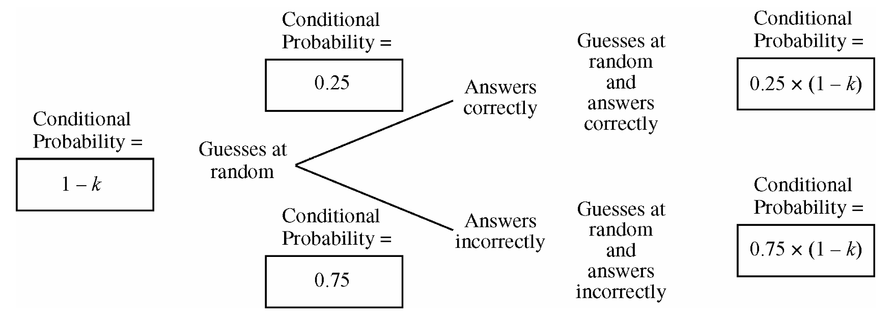
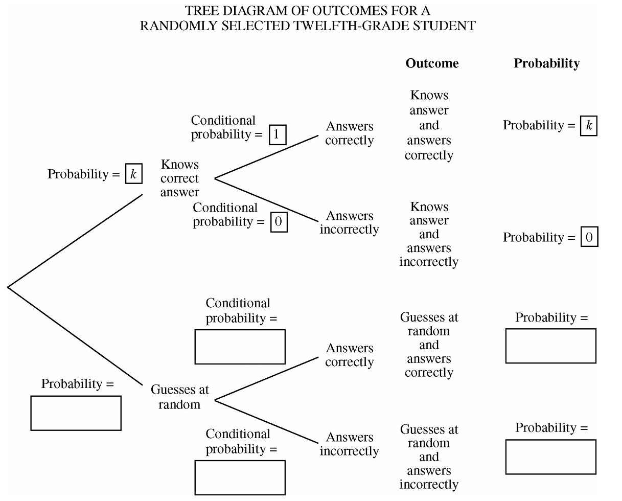
The branches are filled based on the structural logic given in the problem prompt:
• The top initial branch represents the probability a student Knows the answer, which is: $k$
• The bottom initial branch represents the probability a student Does not know the answer, which is: $1 – k$
• Given they know the answer, they choose the correct option with absolute certainty, making the conditional probability of a Correct response: $1$
• Given they do not know the answer, they choose by random guessing out of 4 options, making the conditional probability of a Correct response: $\frac{1}{4} = 0.25$
(c)
To find the overall proportion $p$ of correct answers, accumulate the final correct path terminals from your tree model:
$p = P(\text{Knows}) \times P(\text{Correct} \mid \text{Knows}) + P(\text{Doesn’t Know}) \times P(\text{Correct} \mid \text{Doesn’t Know})$
$p = k(1) + (1-k)(0.25)$
$p = k + 0.25 – 0.25k = 0.75k + 0.25$
(d)
To construct a 99% interval for $k$, isolate $k$ from our part (c) linear transformation model:
$p = 0.75k + 0.25 \implies p – 0.25 = 0.75k \implies k = \frac{p – 0.25}{0.75}$
Now, substitute the lower and upper bounds of $p$ from part (a) into this equation:
$\text{Lower Bound for } k = \frac{0.2682 – 0.25}{0.75} = \frac{0.0182}{0.75} = 0.0243$
$\text{Upper Bound for } k = \frac{0.2918 – 0.25}{0.75} = \frac{0.0418}{0.75} = 0.0557$
The resulting 99% confidence interval for the proportion of students who actually know the answer is $(0.0243, 0.0557)$.
Question
Most-appropriate topic codes (AP Statistics):
• Topic 3.4 — Justifying a Claim Based on a Confidence Interval for a Population Proportion (Part \(\mathrm{a}\))
▶️ Answer/Explanation
(a)
Step 1: Identify the population parameter of interest and the inference procedure by name.
The parameter of interest is \(p\), the true proportion of vaccine-eligible individuals who have high cholesterol levels.
The appropriate procedure is a one-sample \(z\)-interval for a population proportion.
Step 2: Check the required assumptions and conditions for inference.
• The problem states that a random sample of vaccine-eligible individuals was selected, satisfying the randomness condition.
• The large-sample normality condition requires that the number of observed successes and failures are both at least \(10\):
\(n\hat{p} = 978 \ge 10\)
\(n(1-\hat{p}) = 2350 – 978 = 1372 \ge 10\)
Since both values are significantly greater than \(10\), the distribution of the sample proportion can be modeled accurately using a normal curve.
Step 3: Perform the quantitative mechanics of the confidence interval calculation.
The point estimate for the proportion is computed as follows:
\(\hat{p} = \dfrac{978}{2350} \approx 0.4162\)
For a \(99\%\) confidence level, the critical value found from the standard normal table is:
\(z^* = 2.57583\)
The confidence interval formula is:
\(\text{Interval} = \hat{p} \pm z^*\sqrt{\dfrac{\hat{p}(1-\hat{p})}{n}}\)
\(\text{Interval} = 0.41617 \pm 2.57583\sqrt{\dfrac{0.4162(1-0.4162)}{2350}}\)
\(\text{Interval} = 0.41617 \pm 2.57583(0.01017)\)
\(\text{Interval} = 0.41617 \pm 0.02619\)
This yields lower and upper operational boundaries of:
\((0.38998, 0.44236)\)
Step 4: Interpret the resulting confidence interval in the context of the study.
We are \(99\%\) confident that the true proportion of all vaccine-eligible individuals who have high cholesterol levels falls in the interval between \(0.3900\) and \(0.4424\) (or between \(39.0\%\) and \(44.24\%\)).
\(\boxed{(0.38998, 0.44236)}\)
(b)
To guarantee the margin of error is no greater than \(0.02\), we set:
\(z^{*}\sqrt{\dfrac{p(1-p)}{n}} \leq 0.02\)
To be conservative (i.e., to guarantee the condition holds regardless of the true proportion), we use \(p = 0.5\), which maximizes \(p(1-p)\):
\(2.576\sqrt{\dfrac{0.5 \times 0.5}{n}} \leq 0.02\)
Solving for \(n\):
\(\sqrt{\dfrac{0.25}{n}} \leq \dfrac{0.02}{2.576}\)
\(\dfrac{0.25}{n} \leq \left(\dfrac{0.02}{2.576}\right)^{2}\)
\(n \geq \dfrac{(2.576)^{2}(0.5)(0.5)}{(0.02)^{2}} = \dfrac{6.635 \times 0.25}{0.0004} = \dfrac{1.65875}{0.0004} \approx 4{,}147.36\)
\(\boxed{n = 4{,}148}\)
A sample of at least \(\mathbf{4{,}148}\) vaccine-eligible people should be surveyed in Canada.
Question
Most-appropriate topic codes (AP Statistics):
• Topic 3.4 — Justifying a Claim Based on a Confidence Interval for a Population Proportion (Part b)
▶️ Answer/Explanation
(a)
A 95 percent confidence level means that if we were to repeatedly select independent random samples of size $n = 150$ households from this county and construct a 95 percent confidence interval from each sample, then in the long run approximately 95 percent of those generated intervals would successfully capture the true population proportion of households in the county that own at least one dog.
(b)
No. The 95 percent confidence interval $0.417 \pm 0.119$ is the interval $(0.298, 0.536)$. This interval includes the value 0.39 as a plausible value for the population proportion of households in the county that own at least one dog. Therefore, the confidence interval does not provide evidence that the proportion of dog owners in this county is different from the claimed national proportion.
(c)
The sample proportion is 0.417, and the margin of error is 0.119. Determining the sample size requires solving the equation $0.119 = 1.96 \times \sqrt{\dfrac{0.417 \times (1 – 0.417)}{n}}$ for $n$.
Thus, $n = \dfrac{1.96^2 \times 0.417 \times (1 – 0.417)}{0.119^2} \approx 65.95$, so the humane society must have selected 66 households for its sample.
Question
Most-appropriate topic codes (AP Statistics):
• Topic \(3.4\) — Justifying a Claim Based on a Confidence Interval for a Population Proportion (Part \(\mathrm{a}\))
• Topic \(3.2\) — Sampling Distributions for Sample Proportions (Part \(\mathrm{b}\))
▶️ Answer/Explanation
(a)
Procedure: One-sample \(z\)-interval for a population proportion.
Conditions:
Random: The problem states the 50 songs were randomly selected. ✓
Large Counts: \(n\hat{p} = 50 \times 0.26 = 13 \geq 10\) and \(n(1-\hat{p}) = 50 \times 0.74 = 37 \geq 10\). ✓
Both conditions are satisfied, so we may proceed.
Calculation:
The sample proportion is:
\(\hat{p} = \frac{13}{50} = 0.26\)
For a 90% confidence interval, the critical value is \(z^* = 1.645\). The margin of error is:
\(ME = z^* \sqrt{\frac{\hat{p}(1-\hat{p})}{n}} = 1.645 \times \sqrt{\frac{0.26 \times 0.74}{50}}\)
\(ME = 1.645 \times \sqrt{\frac{0.1924}{50}} = 1.645 \times \sqrt{0.003848} = 1.645 \times 0.06203 \approx 0.102\)
The 90% confidence interval is:
\(\hat{p} \pm ME = 0.26 \pm 0.102 = \boxed{(0.158,\ 0.362)}\)
Interpretation: We are 90% confident that the true proportion of all songs on the digital music player that were loaded by Lori is between 0.158 and 0.362.
In plain terms — if we repeated this process many times, about 90% of the confidence intervals we’d construct would capture the actual fraction of songs that Lori loaded. Based on this one interval, our best guess is somewhere between roughly 16% and 36%.
(b)
The distinction between sampling with replacement and without replacement only matters meaningfully when the sample size is large relative to the population size. Here we check the ratio:
\(\frac{\text{Population size}}{\text{Sample size}} = \frac{2384}{50} = 47.7\)
Since the population is about 47.7 times larger than the sample, the sample of 50 represents only:
\(\frac{50}{2384} \approx 2.1\%\text{ of the population}\)
This is well below the standard 10% threshold. When the sample is this small relative to the population, removing a song from the pool (sampling without replacement) barely changes the probability of selecting any remaining song. For example:
Probability of selecting a specific song with replacement: \(\dfrac{1}{2384} \approx 4.195 \times 10^{-4}\)
Probability of selecting a specific song without replacement (after one song removed): \(\dfrac{1}{2383} \approx 4.196 \times 10^{-4}\)
The difference is negligible — on the order of \(10^{-7}\). Because the population is so large relative to the sample, the two sampling methods produce virtually identical results, and the confidence interval from part (a) is valid regardless of which method the player uses.
Question
• Has a high school diploma
Most-appropriate topic codes (AP Statistics):
• Topic 3.3 — Constructing a Confidence Interval for a Population Proportion (Part \(\mathrm{b}\))
• Topic 1.11 — Random Sampling (Part \(\mathrm{c}\))
▶️ Answer/Explanation
(a)
One issue is that random-digit dialing only reaches people who have a telephone. People without a high school diploma tend to have lower-paying jobs, so they may be less likely to be able to afford phone service. As a result, this group could be underrepresented in the sample.
\( \boxed{\text{Households without phones are missed, and these are more likely to lack a diploma, so the estimate may be too low}} \)
(b)
The margin of error for a proportion is
\( ME=z^*\sqrt{\dfrac{p(1-p)}{n}} \)
We want \(ME=0.03\) with \(95\%\) confidence, so \(z^*=1.96\), and we use the pilot estimate \(p=0.22\):
\( 0.03=1.96\sqrt{\dfrac{0.22(0.78)}{n}} \)
Solving for \(n\), first isolate the square root:
\( \sqrt{\dfrac{0.22(0.78)}{n}}=\dfrac{0.03}{1.96} \)
Square both sides:
\( \dfrac{0.22(0.78)}{n}=\left(\dfrac{0.03}{1.96}\right)^2 \)
Solve for \(n\):
\( n=\dfrac{0.22(0.78)}{\left(\dfrac{0.03}{1.96}\right)^2} \)
\( n=\left(\dfrac{1.96}{0.03}\right)^2(0.22)(0.78) \)
\( n\approx 732.47 \)
Since \(n\) must be a whole number and we need at least this many respondents, we round up:
\( \boxed{n=733\text{ respondents}} \)
(c)
A good approach here is stratified random sampling, using each state as a stratum. Within every state, a random sample of adult heads of households would be selected and surveyed, with the sample size in each state chosen based on the precision needed for that state. Once all the state-level samples are collected, the results can be combined to produce an overall national estimate.
\( \boxed{\text{Stratified random sampling — treat each state as a stratum and take a random sample within each state}} \)
Question
Most-appropriate topic codes (AP Statistics):
• Topic 3.3 — Constructing a Confidence Interval for a Population Proportion (Part b)
• Topic 3.4 — Justifying a Claim Based on a Confidence Interval for a Population Proportion (Parts c, d)
▶️ Answer/Explanation
(a)
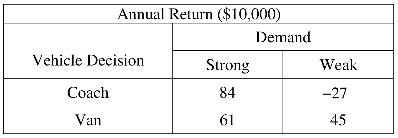
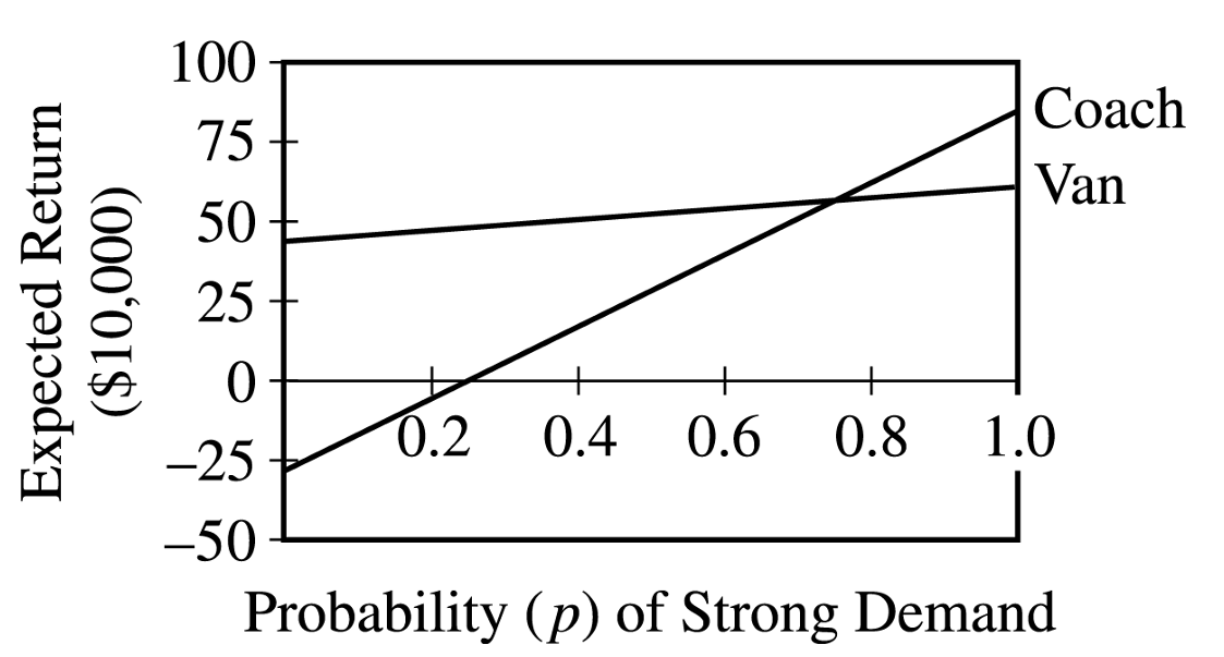
Looking at the graph, the line for vans starts higher than the line for coaches when \(p\) is small (since vans don’t lose much money even in a weak market), but the coach line rises more steeply and eventually overtakes the van line at \(p=0.76\). For any \(p\) less than \(0.76\), the van line sits above the coach line, meaning vans give the larger expected return.
We can also confirm this algebraically by plugging in a value of \(p\) less than \(0.76\), say \(p=0.5\):
Expected return for coaches:
\( 111(0.5)-27=55.5-27=28.5 \)
So the coach return is \(\$285{,}000\).
Expected return for vans:
\( 16(0.5)+45=8+45=53 \)
So the van return is \(\$530{,}000\).
Since \(53>28.5\), vans give the higher expected return at \(p=0.5\). Because both expected-return equations are linear in \(p\) and the two lines cross only once (at \(p=0.76\)), this same ordering — vans above coaches — must hold for every value of \(p\) below \(0.76\).
\( \boxed{\text{For } p<0.76, \text{ vans provide the greater expected annual return.}} \)
(b)
Since we’re estimating the proportion \(p\) of similar markets with strong demand based on a sample proportion, this calls for a one-sample \(z\)-confidence interval for a proportion.
From the sample,
\( \hat{p}=\dfrac{65}{100}=0.65 \)
Before building the interval, check the conditions. The \(100\) markets were a random sample, and since there are several thousand similar markets nationally, \(100\) is less than \(10\%\) of that population. For the large-sample condition,
\( n\hat{p}=100(0.65)=65 \)
\( n(1-\hat{p})=100(0.35)=35 \)
Both of these are well above \(10\), so a normal approximation is reasonable and the interval can proceed.
The formula for the confidence interval is:
\( \hat{p}\pm z^{*}\sqrt{\dfrac{\hat{p}(1-\hat{p})}{n}} \)
Compute the standard error first:
\( \sqrt{\dfrac{(0.65)(0.35)}{100}}=\sqrt{\dfrac{0.2275}{100}}=\sqrt{0.002275} \)
\( \approx0.0477 \)
For \(95\%\) confidence, \(z^{*}=1.96\), so the margin of error is:
\( 1.96\times0.0477\approx0.0935 \)
Putting it together:
\( 0.65\pm0.0935 \)
\( \boxed{(0.5565,\ 0.7435)} \)
Interpretation: We can be \(95\%\) confident that the true proportion of similar markets that will experience strong demand is between about \(0.56\) and \(0.74\).
(c)
The interval from part (b) tells us that the plausible values for \(p\), the probability of strong demand, range from about \(0.56\) to \(0.74\). Every single value in that interval is less than \(0.76\), the cutoff found in part (a). Since part (a) showed that vans produce a larger expected return than coaches whenever \(p<0.76\), this means that for every plausible value of \(p\) suggested by the data, vans come out ahead. So choosing vans makes sense — it’s the decision that’s expected to perform better across the entire range of demand probabilities that the sample data support.
(d)
Even though the entire confidence interval lies below \(0.76\), the vice president could argue based on the actual dollar amounts at stake rather than just which option has the slightly higher expected return. Notice that throughout the confidence interval \((0.56,\ 0.74)\), the probability of strong demand is consistently estimated to be greater than \(0.5\) — meaning strong demand is more likely than weak demand in this market.
If demand turns out to be strong, the payoff table shows coaches return \(\$840{,}000\) compared to only \(\$610{,}000\) for vans — a substantial difference in the company’s favor. Meanwhile, if demand is weak, coaches lose \(\$270{,}000\) while vans still make \(\$450{,}000\), but this weak-demand scenario is the less likely one according to the interval. So the vice president could reasonably argue that, since strong demand is more probable and the upside for coaches in that case is so much larger than the modest expected-value edge vans have overall, coaches are actually the better choice for this particular route.
Question

Most-appropriate topic codes (AP Statistics):
• Topic 3.4 — Justifying a Claim Based on a Confidence Interval for a Population Proportion (Part a)
• Topic 3.1 — Estimators (Part b)
• Topic 3.2 — Sampling Distributions for Sample Proportions (Parts b, c)
▶️ Answer/Explanation
(a)
Procedure and Conditions:
We use a one-sample \(z\)-confidence interval for a proportion: \(\hat{p} \pm z^* \sqrt{\dfrac{\hat{p}(1-\hat{p})}{n}}\).
From the table, the sample of females in the 40–44 age-group has \(n = 370\). With 10% contracting the illness, \(\hat{p} = 0.10\).
Check conditions: The sample is a random sample from the HMO population. The expected number of successes is \(n\hat{p} = 370(0.10) = 37 > 5\) and the expected number of failures is \(n(1-\hat{p}) = 370(0.90) = 333 > 5\), so the sample size is large enough to proceed.
Mechanics:
\( \hat{p} \pm z^* \sqrt{\frac{\hat{p}(1-\hat{p})}{n}} = 0.10 \pm 1.96\sqrt{\frac{(0.10)(0.90)}{370}} \)
\( = 0.10 \pm 1.96\sqrt{\frac{0.09}{370}} = 0.10 \pm 1.96(0.01559) = 0.10 \pm 0.0306 \)
\( \boxed{(0.06943,\ 0.13057)} \)
Interpretation of the confidence interval:
We are 95% confident that the true proportion of the HMO’s 40–44 year old female patients who would contract this illness is between approximately 0.069 and 0.131 (i.e., between about 6.9% and 13.1%).
Interpretation of the 95% confidence level:
If we were to take many random samples of size 370 from this population and compute a 95% confidence interval from each sample, approximately 95% of those intervals would capture the true population proportion of 40–44 year old female HMO patients who contract the illness. In other words, the method we used to construct this interval will fail to contain the true proportion only about 5% of the time in repeated sampling.
(b)
The width of a confidence interval for a proportion is determined by the margin of error \(z^*\sqrt{\dfrac{\hat{p}(1-\hat{p})}{n}}\), which depends on both \(\hat{p}\) and \(n\).
When the sample proportions are equal (both 0.10), the only factor causing different interval widths is the different sample sizes — females had \(n = 370\) while males had \(n = 230\) in the 40–44 group, producing a wider interval for males.
To make the confidence interval widths equal for all 8 groups when sample proportions are equal, the sample sizes for all 8 groups must be equal.
With 2,000 total subjects and 8 groups, each group should receive a sample of size:
\( n = \frac{2000}{8} = \boxed{250 \text{ subjects per group}} \)
Equal sample sizes guarantee equal standard errors (and therefore equal interval widths) whenever the sample proportions are the same.
(c)
When sample proportions differ across groups, equal widths require not equal sample sizes but rather sample sizes proportional to \(\hat{p}(1-\hat{p})\) for each group — this keeps the standard error \(\sqrt{\dfrac{\hat{p}(1-\hat{p})}{n}}\) the same across all groups.
Compute \(p(1-p)\) for each age-group using the anticipated proportions: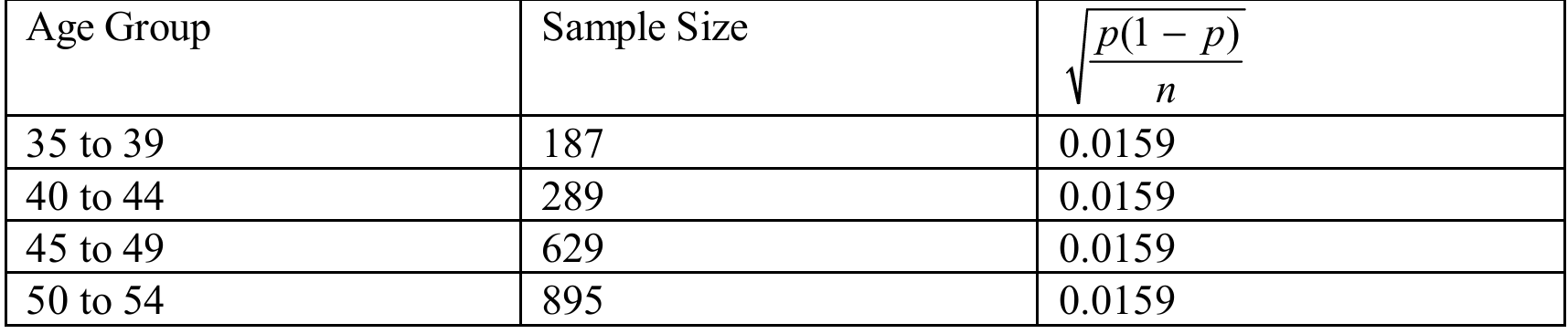
The total of all \(p(1-p)\) values is:
\( 0.0475 + 0.0736 + 0.1600 + 0.2275 = 0.5086 \)
Allocate the 2,000 subjects proportionally:
\( n_{35\text{-}39} = \frac{0.0475}{0.5086} \times 2000 = \boxed{186.79} \)
\( n_{40\text{-}44} = \frac{0.0736}{0.5086} \times 2000 = \boxed{289.42} \)
\( n_{45\text{-}49} = \frac{0.1600}{0.5086} \times 2000 = \boxed{629.18} \)
\( n_{50\text{-}54} = \frac{0.2275}{0.5086} \times 2000 = \boxed{894.61} \)
These four sample sizes sum to 2,000 and ensure that \(\sqrt{\dfrac{p(1-p)}{n}}\) is approximately equal across all four age-groups, producing confidence intervals of equal width.