AP Statistics 3.7 Carrying Out a Test for a Population Proportion- Exam Style Questions - FRQs - New Syllabus

Question

A software application (app) lets users enter questions to receive answers in the form of images, texts, or videos. Research indicates that 22 percent of high school students in Country W use the app to help them with their homework at least once per week. Karen is an AP Statistics student in Country W at a high school that has more than 2,000 students. She believes the proportion of all students at her school who use the app to help them with their homework at least once per week is greater than the proportion for her country. To investigate her belief, she took a simple random sample of 130 students from her school and found that 38 of the sampled students use the app to help them with their homework at least once per week.

Is there convincing statistical evidence, at a 0.05 significance level, to support Karen’s belief? Justify your answer with the appropriate inference procedure.

Most-appropriate topic codes (AP Statistics):

• Topic $3.5$ — Setting Up a Test for a Population Proportion (Entire Question)
• Topic $3.6$ — $p$-Values (Entire Question)
• Topic $3.7$ — Carrying Out a Test for a Population Proportion (Entire Question)

▶️ Answer/Explanation

Step 1: State the Hypotheses and Define the Parameter
Let $p$ represent the true proportion of all students at Karen’s high school who use the application to help them with their homework at least once per week.
$H_0: p = 0.22$
$H_a: p > 0.22$

Step 2: Identify the Procedure and Check Conditions
The appropriate procedure is a one-sample $z$-test for a population proportion.
• Randomness: Karen selected a simple random sample of 130 students from her high school.
• Independence (10% Rule): The sample size of $n = 130$ is less than 10% of the total high school population, which is stated to be greater than 2,000 students ($130 \le 0.10 \times 2,000 = 200$).
• Large Counts Condition: Assuming $H_0$ is true, the expected number of successes is $n p_0 = 130 \times 0.22 = 28.6$ and the expected number of failures is $n(1 – p_0) = 130 \times (1 – 0.22) = 101.4$. Since both values are at least 10 ($28.6 \ge 10$ and $101.4 \ge 10$), a normal distribution can be used to model the sampling distribution of the sample proportion.

Step 3: Calculate the Test Statistic and $p$-value
The sample proportion is $\hat{p} = \dfrac{38}{130} \approx 0.2923$.
The standard error of the sampling distribution is $\sigma_{\hat{p}} = \sqrt{\dfrac{p_0(1 – p_0)}{n}} = \sqrt{\dfrac{0.22 \times 0.78}{130}} = \sqrt{\dfrac{0.1716}{130}} \approx 0.0363$.
The test statistic is $z = \dfrac{\hat{p} – p_0}{\sigma_{\hat{p}}} = \dfrac{0.2923 – 0.22}{0.0363} \approx 1.99$.
The $p$-value for this one-tailed right test is $P(Z > 1.99) = 1 – 0.9767 = 0.0233$.

Step 4: Formulate the Conclusion
• Because the computed $p$-value ($0.0233$) is less than the significance level $\alpha = 0.05$, we reject the null hypothesis $H_0$.
• There is convincing statistical evidence to support Karen’s belief that the proportion of all students at her high school who use the app to help them with their homework at least once per week is greater than the national proportion of 0.22.

Question

The manager of a large company that sells pet supplies online wants to increase sales by encouraging repeat purchases. The manager believes that if past customers are offered $\$10$ off their next purchase, more than $40 \text{ percent}$ of them will place an order. To investigate the belief, $90$ customers who placed an order in the past year are selected at random. Each of the selected customers is sent an e-mail with a coupon for $\$10$ off the next purchase if the order is placed within $30$ days. Of those who receive the coupon, $38$ place an order.

(a) Is there convincing statistical evidence, at the significance level of $\alpha=0.05$, that the manager’s belief is correct? Complete the appropriate inference procedure to support your answer.

(b) Based on your conclusion from part (a), which of the two errors, Type I or Type II, could have been made? Interpret the consequence of the error in context.

Most-appropriate topic codes (AP Statistics):

• Topic $3.5$ — Setting Up a Test for a Population Proportion (Part $ \mathrm{a} $)
• Topic $3.6$ — $p$-Values (Part $ \mathrm{a} $)
• Topic $3.7$ — Carrying Out a Test for a Population Proportion (Part $ \mathrm{a} $)
• Topic $3.11$ — Justifying a Claim Based on a Confidence Interval for the Difference Between Two Population Proportions (Part $ \mathrm{b} $)

▶️ Answer/Explanation

(a)
Let $p$ be the true proportion of customers who place an order. We test $H_0: p = 0.40$ against $H_a: p > 0.40$.
Conditions are met: it’s a random sample, the $10\%$ rule is satisfied (assume $\ge 900$ customers), and expected counts $(36, 54)$ are both $\ge 10$.
The sample proportion is $\hat{p} = \frac{38}{90} \approx 0.422$, giving a test statistic $z = \frac{0.422 – 0.40}{\sqrt{0.4(0.6)/90}} \approx 0.430$ and a $p$-value of $0.333$.
Since $0.333 > 0.05$, we fail to reject $H_0$; there is not convincing evidence the manager’s belief is correct.

(b)
Because we failed to reject the null hypothesis, a Type II error could have been made.
In context, this means the manager incorrectly thinks the coupon won’t bring in more than $40\%$ of customers, deciding not to use it and ultimately missing out on a promotion that would have increased sales.

Question

A city council wants to estimate the proportion of adult residents who are able to pass a standard physical fitness test. A random sample of 48 adults was selected, and each person was given the fitness test. Of the 48 adults sampled, 20 were able to pass the test.

The city council will provide funding for a new fitness center if there is convincing evidence that less than 35 percent of all adult residents are able to pass the physical fitness test. Let $p$ represent the proportion of all adult residents in the city who are able to pass the physical fitness test.

(a) In the context of this study, describe a Type II error and its consequence.

(b) The city council decided to test the hypotheses $H_0: p = 0.35$ versus $H_a: p < 0.35$ using their sample data. The data resulted in a $p$-value of 0.97. What conclusion should the city council draw?

(c) After seeing the results of the survey, a council member remarked that the sample was flawed because it was recruited by asking for volunteers from a local running club, rather than choosing a completely random sample of city residents. Describe how this flaw would affect the inference about the proportion of all adult residents who can pass the test.

Most-appropriate topic codes (AP Statistics):

• Topic 3.8 — Potential Errors When Performing Tests (Part a)
• Topic 3.5 — Setting Up a Test for a Population Proportion (Part b)
• Topic 3.6 — p-Values (Part b)
• Topic 3.7 — Carrying Out a Test for a Population Proportion (Part b)
• Topic 1.12 — Potential Problems with Sampling (Part c)

▶️ Answer/Explanation

(a)
In the context of the study, a Type II error means failing to reject the null hypothesis that 35 percent of adult residents in the city are able to pass the fitness test when, in reality, the true proportion who can pass is actually less than 35 percent.
The real-world consequence of this error is that the city council would decide not to build or fund the new fitness center, even though the community actually needs it because the general health level is lower than desired.

(b)
Because the $p$-value of $0.97$ is much larger than standard significance levels like $\alpha = 0.05$, the council should fail to reject the null hypothesis.
There is not enough convincing evidence to conclude that the true proportion of adult residents in the city who can pass the test is less than 35 percent.
In fact, the observed sample proportion is:
$\hat{p} = \dfrac{20}{48} \approx 0.417$
Since $0.417$ is actually higher than the baseline value of $0.35$, it shifts in the opposite direction of what the alternative hypothesis was trying to establish.

(c)
Recruiting volunteers from a local running club creates a non-random, heavily biased sample because runners are typically in much better physical condition than the general public.
Consequently, the sample proportion of success $\hat{p} = 0.417$ is almost certainly an overestimation of the true proportion $p$ for all city residents.
This makes any resulting inference invalid, as it hides the true lack of physical fitness among the broader city population and could mistakenly convince the council that a new fitness center is unnecessary.

Question

For many years, the medically accepted practice of giving aid to a person experiencing a heart attack was to have the person who placed the emergency call administer chest compression (CC) plus standard mouth-to-mouth resuscitation (MMR) to the heart attack patient until the emergency response team arrived. However, some researchers believed that CC alone would be a more effective approach.

In the 1990s a study was conducted in Seattle in which 518 cases were randomly assigned to treatments: 278 to CC plus standard MMR and 240 to CC alone. A total of 64 patients survived the heart attack: 29 in the group receiving CC plus standard MMR, and 35 in the group receiving CC alone. A test of significance was conducted on the following hypotheses.

$H_0$: The survival rates for the two treatments are equal.
$H_a$: The treatment that uses CC alone produces a higher survival rate.

This test resulted in a $p$-value of 0.0761.

(a) Interpret what this $p$-value measures in the context of this study.

(b) Based on this $p$-value and study design, what conclusion should be drawn in the context of this study? Use a significance level of $\alpha = 0.05$.

(c) Based on your conclusion in part (b), which type of error, Type I or Type II, could have been made? What is one potential consequence of this error?

Most-appropriate topic codes (AP Statistics):

• Topic $3.6$ — p-Values (Part $\mathrm{a}$)
• Topic $3.7$ — Carrying Out a Test for a Population Proportion (Part $\mathrm{b}$)
• Topic $3.8$ — Potential Errors When Performing Tests (Part $\mathrm{c}$)

▶️ Answer/Explanation

(a)
The $p$-value of $0.0761$ is the probability of observing a difference between the two sample survival proportions
$ \hat{p}_{\text{CC}} – \hat{p}_{\text{CC+MMR}} $
as large as or larger than the one actually observed in this study ($\frac{35}{240} – \frac{29}{278}$), assuming that the survival rates for the two treatments are truly equal in the population.
In plain terms: if CC alone and CC + MMR actually produce the same survival rate, there is still about a $7.61\%$ chance of seeing the CC-alone group outperform the CC + MMR group by as much as (or more than) it did in this study just by random chance alone.

(b)
Compare the $p$-value to the significance level:
$ p\text{-value} = 0.0761 > \alpha = 0.05 $
Because the $p$-value exceeds $\alpha$, we fail to reject $H_0$.
There is not sufficient evidence at the $\alpha = 0.05$ significance level to conclude that the treatment using CC alone produces a higher survival rate than CC plus standard MMR for heart attack patients.
Note that since the 518 cases were randomly assigned to the two treatments, this is a properly designed experiment — so a significant result would have allowed a causal conclusion. However, since we fail to reject $H_0$, we simply cannot make that claim here.

(c)
Because we failed to reject $H_0$ in part (b), the only error that could have occurred is a Type II error — failing to reject a null hypothesis that is actually false.
In this context, a Type II error would mean that CC alone truly does produce a higher survival rate than CC + MMR, but the study did not provide enough evidence to detect it.
A potential consequence of this error is that the medical community would continue recommending CC plus MMR as the standard treatment for heart attack patients, even though CC alone would actually save more lives. Heart attack patients would receive a less effective treatment, leading to preventable deaths that would not have occurred had CC alone been adopted as the standard practice.

Question

Sunshine Farms wants to know whether there is a difference in consumer preference for two new juice products — Citrus Fresh and Tropical Taste. In an initial blind taste test, 8 randomly selected consumers were given unmarked samples of the two juices. The product that each consumer tasted first was randomly decided by the flip of a coin. After tasting the two juices, each consumer was asked to choose which juice he or she preferred, and the results were recorded.

(a) Let $p$ represent the population proportion of consumers who prefer Citrus Fresh. In terms of $p$, state the hypotheses that Sunshine Farms is interested in testing.

(b) One might consider using a one-proportion $z$-test to test the hypotheses in part (a). Explain why this would not be a reasonable procedure for this sample.

(c) Let $X$ represent the number of consumers in the sample who prefer Citrus Fresh. Assuming there is no difference in consumer preference, find the probability for each possible value of $X$. Record the $x$-values and the corresponding probabilities in the table below.

(d) When testing the hypotheses in part (a), Sunshine Farms will conclude that there is a consumer preference if too many or too few individuals prefer Citrus Fresh. Based on your probabilities in part (c), is it possible for the significance level (probability of rejecting the null hypothesis when it is true) for this test to be exactly 0.05? Justify your answer.

(e) The preference data for the 8 randomly selected consumers are given in the table below.

Based on these preferences and your previous work, test the hypotheses in part (a).

(f) Sunshine Farms plans to add one of these two new juices — Citrus Fresh or Tropical Taste — to its production schedule. A follow-up study will be conducted to decide which of the two juices to produce. Make one recommendation for the follow-up study that would make it better than the initial study. Provide a statistical justification for your recommendation in the context of the problem.

Most-appropriate topic codes (AP Statistics):

• Topic 3.5 — Setting Up a Test for a Population Proportion (Part $\mathrm{a}$)
• Topic 3.2 — Sampling Distributions for Sample Proportions (Part $\mathrm{b}$)
• Topic 2.10 — The Binomial Distribution (Part $\mathrm{c}$)
• Topic 3.6 — p-Values (Part $\mathrm{d}$)
• Topic 3.7 — Carrying Out a Test for a Population Proportion (Part $\mathrm{e}$)
• Topic 1.13 — Experimental Design (Part $\mathrm{f}$)

▶️ Answer/Explanation

(a)
Let $p$ be the population proportion of consumers who prefer Citrus Fresh. The hypotheses are:
$H_0: p = 0.5$
$H_a: p \neq 0.5$
A two-sided alternative is appropriate because Sunshine Farms wants to detect any difference in preference, not just preference for one particular juice.

(b)
The conditions for a one-proportion $z$-test require that both $np$ and $n(1-p)$ be at least 5 (or 10). Here:
$np = 8 \times 0.5 = 4 < 5$
$n(1-p) = 8 \times 0.5 = 4 < 5$
Since both values are less than 5, the large-sample normal approximation is not valid, and using a one-proportion $z$-test would not be appropriate for a sample of only $n = 8$.

(c)
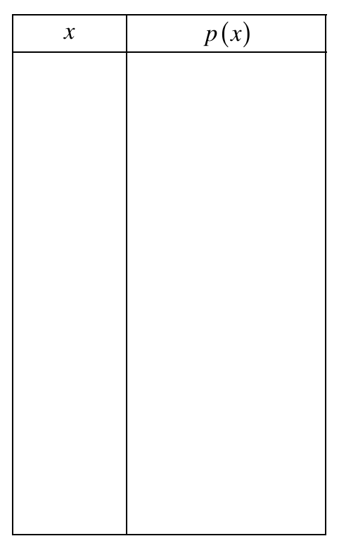
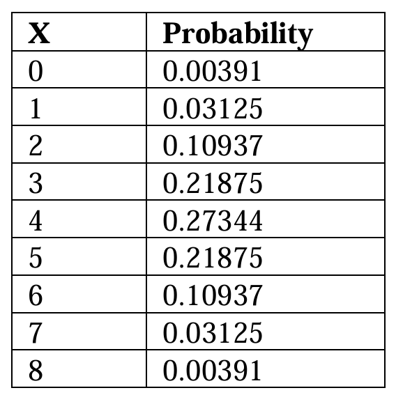
Under $H_0$, $X \sim \text{Binomial}(n = 8,\ p = 0.5)$. The probabilities are computed using:
$P(X = x) = \binom{8}{x}(0.5)^x(0.5)^{8-x} = \binom{8}{x}(0.5)^8$

(d)
No, it is not possible for the significance level to be exactly 0.05. Because $X$ is a discrete random variable, the tail probabilities can only take specific values — there is no rejection region that gives a type I error probability of exactly 0.05.
The most extreme rejection region $(X = 0 \text{ or } X = 8)$ gives:
$\alpha = 2 \times 0.00391 = 0.00782 < 0.05$
The next possible rejection region $(X \leq 1 \text{ or } X \geq 7)$ gives:
$\alpha = 2 \times (0.00391 + 0.03125) = 2 \times 0.03516 = 0.07031 > 0.05$
Since no rejection region produces a type I error probability of exactly 0.05, a significance level of exactly 0.05 is not achievable with this test.
$\boxed{\alpha = 0.05 \text{ is not achievable — the achievable levels jump from } 0.00782 \text{ to } 0.07031}$

(e)
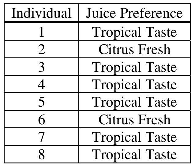
From the data, 2 out of 8 consumers preferred Citrus Fresh, so $X = 2$.
Since this is a two-sided test, the $p$-value is the probability of observing a result at least as extreme as $X = 2$ in either tail:
$p\text{-value} = P(X \leq 2) + P(X \geq 6)$
$= 2 \times [P(X=0) + P(X=1) + P(X=2)]$
$= 2 \times (0.00391 + 0.03125 + 0.10937)$
$= 2 \times 0.14453 = 0.28906$
Since the $p$-value of $0.289$ is much larger than any reasonable significance level (e.g., $\alpha = 0.05$ or $\alpha = 0.07031$), we fail to reject $H_0$. There is not statistically significant evidence of a consumer preference between Citrus Fresh and Tropical Taste.
$\boxed{p\text{-value} \approx 0.289 \implies \text{Fail to reject } H_0; \text{ no significant consumer preference detected}}$

(f)
The most important recommendation is to increase the number of consumers in the study. With only $n = 8$ consumers, the test has very low power — even a large true difference in preference (like 75% vs. 25%) may not produce a statistically significant result. Increasing the sample size would reduce the standard error of the estimated proportion $\hat{p}$, making it easier to detect a real difference, and would allow the use of the large-sample one-proportion $z$-test since $np \geq 5$ and $n(1-p) \geq 5$ would be satisfied. For example, with $n = 80$ and $X = 20$ (same sample proportion of 0.25), the $z$-statistic would be approximately:
$z = \frac{0.25 – 0.5}{\sqrt{\frac{0.5(0.5)}{80}}} \approx -4.47$
which gives a $p$-value near zero, allowing a clear conclusion to be reached.
$\boxed{\text{Recommendation: Increase sample size to increase power and enable use of the } z\text{-test}}$

Question

Some boxes of a certain brand of breakfast cereal include a voucher for a free video rental inside the box. The company that makes the cereal claims that a voucher can be found in 20 percent of the boxes. However, based on their experiences eating this cereal at home, a group of students believes that the proportion of boxes with vouchers is less than 0.2. This group of students purchased 65 boxes of the cereal to investigate the company’s claim. The students found a total of 11 vouchers for free video rentals in the 65 boxes.

Suppose it is reasonable to assume that the 65 boxes purchased by the students are a random sample of all boxes of this cereal. Based on this sample, is there support for the students’ belief that the proportion of boxes with vouchers is less than $0.2$? Provide statistical evidence to support your answer.

Most-appropriate topic codes (AP Statistics):

• Topic 3.5 — Setting Up a Test for a Population Proportion (hypotheses)
• Topic 3.7 — Carrying Out a Test for a Population Proportion (conditions, mechanics, conclusion)
• Topic 3.6 — p-Values (interpretation of statistical evidence)

▶️ Answer/Explanation

Step 1: Hypotheses
Let $p$ = the true proportion of boxes of this cereal that contain a voucher.
$ H_0: p=0.2 $
$ H_a: p<0.2 $

Step 2: Test and conditions
This is a one-sample $z$-test for a proportion:
$ z=\dfrac{\hat{p}-p_0}{\sqrt{\dfrac{p_0(1-p_0)}{n}}} $
Checking conditions:
$ np_0=65(0.2)=13\ge 10 $
$ n(1-p_0)=65(0.8)=52\ge 10 $
It’s reasonable that there are at least $650$ boxes of this cereal in total, so the $10\%$ condition is met, and the stem tells us the sample is random, so the observations are independent.

Step 3: Mechanics
The sample proportion is
$ \hat{p}=\dfrac{11}{65}\approx 0.169 $
The test statistic is
$ z=\dfrac{0.169-0.2}{\sqrt{\dfrac{0.2(1-0.2)}{65}}} $
$ z\approx -0.62 $
The corresponding p-value is
$ P(Z<-0.62)\approx 0.2676 $
$ \boxed{z\approx -0.62,\quad p\text{-value}\approx 0.2676} $

Step 4: Conclusion
A p-value of $0.2676$ is large — much bigger than any typical significance level like $0.05$. This means a sample proportion as low as $0.169$ wouldn’t be at all surprising if the true proportion really were $0.2$, so there isn’t enough evidence to reject the company’s claim.
$ \boxed{\text{Since the p-value (0.2676) is large, we fail to reject } H_0\text{ — no significant evidence that } p<0.2} $

AP Statistics 3.7 Carrying Out a Test for a Population Proportion- Exam Style Questions - FRQs - New Syllabus

Question

Question

Question

Question

Question

Question

Resources

Members

Company