
AP Statistics 3.8 Potential Errors When Performing Tests- Exam Style Questions - FRQs - New Syllabus
Question
A city council wants to estimate the proportion of adult residents who are able to pass a standard physical fitness test. A random sample of 48 adults was selected, and each person was given the fitness test. Of the 48 adults sampled, 20 were able to pass the test.
Most-appropriate topic codes (AP Statistics):
• Topic 3.5 — Setting Up a Test for a Population Proportion (Part b)
• Topic 3.6 — p-Values (Part b)
• Topic 3.7 — Carrying Out a Test for a Population Proportion (Part b)
• Topic 1.12 — Potential Problems with Sampling (Part c)
▶️ Answer/Explanation
(a)
In the context of the study, a Type II error means failing to reject the null hypothesis that 35 percent of adult residents in the city are able to pass the fitness test when, in reality, the true proportion who can pass is actually less than 35 percent.
The real-world consequence of this error is that the city council would decide not to build or fund the new fitness center, even though the community actually needs it because the general health level is lower than desired.
(b)
Because the \(p\)-value of \(0.97\) is much larger than standard significance levels like \(\alpha = 0.05\), the council should fail to reject the null hypothesis.
There is not enough convincing evidence to conclude that the true proportion of adult residents in the city who can pass the test is less than 35 percent.
In fact, the observed sample proportion is:
\(\hat{p} = \dfrac{20}{48} \approx 0.417\)
Since \(0.417\) is actually higher than the baseline value of \(0.35\), it shifts in the opposite direction of what the alternative hypothesis was trying to establish.
(c)
Recruiting volunteers from a local running club creates a non-random, heavily biased sample because runners are typically in much better physical condition than the general public.
Consequently, the sample proportion of success \(\hat{p} = 0.417\) is almost certainly an overestimation of the true proportion \(p\) for all city residents.
This makes any resulting inference invalid, as it hides the true lack of physical fitness among the broader city population and could mistakenly convince the council that a new fitness center is unnecessary.
Question
Most-appropriate topic codes (AP Statistics):
• Topic 3.15 — Carrying Out a Chi-Square Test for Homogeneity or Independence (Part b)
• Topic 3.15 — Carrying Out a Chi-Square Test for Homogeneity or Independence (Part c)
• Topic 3.8 — Potential Errors When Performing Tests (Part d)
▶️ Answer/Explanation
(a)
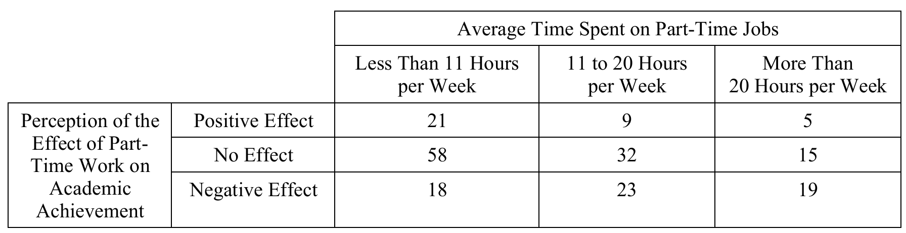
\(H_0\): There is no association between the perceived effect of part-time work on academic achievement and the average time spent on part-time jobs.
\(H_a\): There is an association between the perceived effect of part-time work on academic achievement and the average time spent on part-time jobs.
(b)
The conditions for a chi-square inference procedure are met for these data:
1. Randomization: The problem states that the advisory board surveyed a “simple random sample” of students, so the random condition is met.
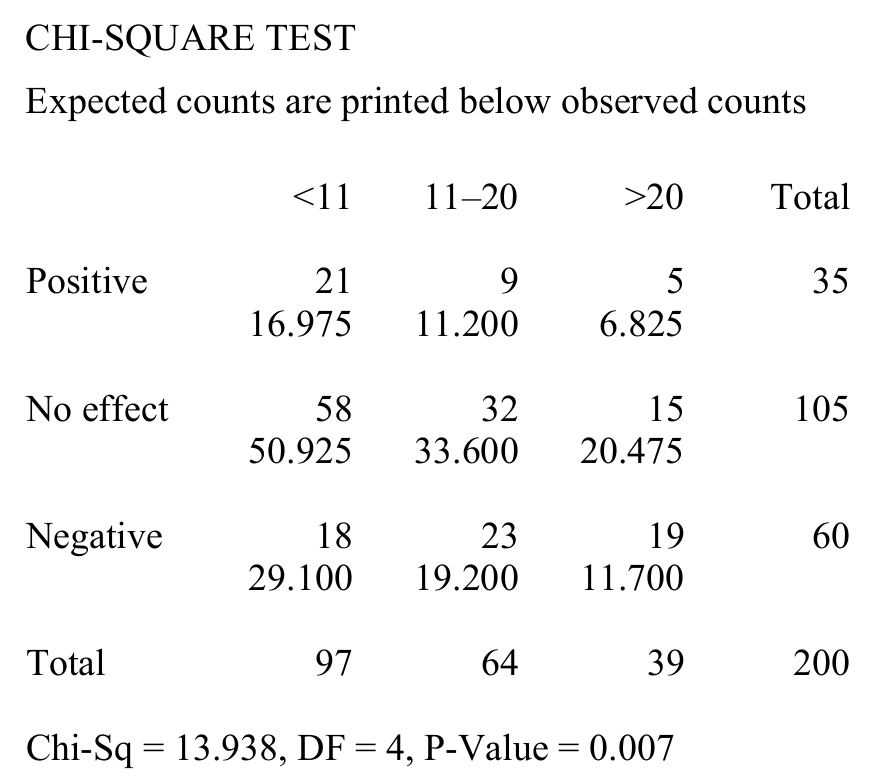
2. Expected Counts: All expected cell counts must be at least \(5\). Looking at the provided computer output, the expected counts (printed below the observed counts) are all greater than \(5\). The smallest expected count is \(6.825\), so this condition is met.
(c)
Because the \(p\)-value of \(0.007\) is less than standard significance levels (like \(\alpha = 0.05\)), we reject the null hypothesis.
The advisory board should conclude that there is convincing statistical evidence of an association between a student’s perceived effect of part-time work on academic achievement and the average number of hours per week that the student works.
(d)
Because the null hypothesis was rejected in part (c), the advisory board might have made a Type I error.
In the context of the question, a Type I error would be concluding that there is an association between the perceived effect of part-time work on academic achievement and the average time spent on part-time jobs when, in reality, there is no such association between these two variables.
Question
\(H_a\): The treatment that uses CC alone produces a higher survival rate.
Most-appropriate topic codes (AP Statistics):
• Topic \(3.7\) — Carrying Out a Test for a Population Proportion (Part \(\mathrm{b}\))
• Topic \(3.8\) — Potential Errors When Performing Tests (Part \(\mathrm{c}\))
▶️ Answer/Explanation
(a)
The \(p\)-value of \(0.0761\) is the probability of observing a difference between the two sample survival proportions
\( \hat{p}_{\text{CC}} – \hat{p}_{\text{CC+MMR}} \)
as large as or larger than the one actually observed in this study (\(\frac{35}{240} – \frac{29}{278}\)), assuming that the survival rates for the two treatments are truly equal in the population.
In plain terms: if CC alone and CC + MMR actually produce the same survival rate, there is still about a \(7.61\%\) chance of seeing the CC-alone group outperform the CC + MMR group by as much as (or more than) it did in this study just by random chance alone.
(b)
Compare the \(p\)-value to the significance level:
\( p\text{-value} = 0.0761 > \alpha = 0.05 \)
Because the \(p\)-value exceeds \(\alpha\), we fail to reject \(H_0\).
There is not sufficient evidence at the \(\alpha = 0.05\) significance level to conclude that the treatment using CC alone produces a higher survival rate than CC plus standard MMR for heart attack patients.
Note that since the 518 cases were randomly assigned to the two treatments, this is a properly designed experiment — so a significant result would have allowed a causal conclusion. However, since we fail to reject \(H_0\), we simply cannot make that claim here.
(c)
Because we failed to reject \(H_0\) in part (b), the only error that could have occurred is a Type II error — failing to reject a null hypothesis that is actually false.
In this context, a Type II error would mean that CC alone truly does produce a higher survival rate than CC + MMR, but the study did not provide enough evidence to detect it.
A potential consequence of this error is that the medical community would continue recommending CC plus MMR as the standard treatment for heart attack patients, even though CC alone would actually save more lives. Heart attack patients would receive a less effective treatment, leading to preventable deaths that would not have occurred had CC alone been adopted as the standard practice.
Question
Most-appropriate topic codes (AP Statistics):
• Topic 4.4 — Setting Up a Test for a Population Mean or Population Mean Difference (Part \(\mathrm{b}\))
• Topic 3.8 — Potential Errors When Performing Tests (Part \(\mathrm{b}\))
▶️ Answer/Explanation
(a)
Proposed Design (Completely Randomized Design):
Assign each of the 100 patients a unique number from 00 to 99. Using a random number table (or random number generator), select 50 unique numbers. The patients corresponding to the selected numbers will form Group 1 (Music Treatment); the remaining 50 patients will form Group 2 (Control — Noise-Free Environment).
Measure the diastolic blood pressure of every patient before the treatment begins. Then:
Group 1 patients sit quietly in a room where soothing music is played for 20 minutes.
Group 2 patients sit quietly in a noise-free environment for 20 minutes.
At the end of the 20-minute period, measure the diastolic blood pressure of every patient again. Compute the reduction in diastolic blood pressure (before \(-\) after) for each patient. Run a two-sample \(t\)-test to compare the mean reduction in the two groups.
Alternatively (Paired Design):
Each patient receives both treatments on two separate occasions, with a suitable washout period in between. For each patient, flip a coin to randomly assign which treatment is administered first. Compute the difference (music reduction \(-\) noise-free reduction) for each patient, and use a paired \(t\)-test to determine whether the mean difference is significantly greater than zero.
(b)
Let \(\mu_M\) = mean reduction in diastolic blood pressure under the music treatment, and \(\mu_C\) = mean reduction under the control (noise-free) treatment. The hypotheses are:
\(H_0: \mu_M = \mu_C \qquad H_a: \mu_M > \mu_C\)
Type I Error:
Rejecting \(H_0\) when it is actually true — that is, concluding that soothing music does reduce diastolic blood pressure more than sitting quietly, when in reality it does not.
Consequence: The clinic will offer music therapy as a free service to its patients even though the therapy is ineffective. This wastes clinic resources and money, providing no real medical benefit to patients.
Type II Error:
Failing to reject \(H_0\) when it is actually false — that is, concluding that soothing music does not reduce diastolic blood pressure more than sitting quietly, when in reality it does.
Consequence: The clinic will not offer music therapy, even though the therapy would genuinely help patients reduce their blood pressure. Patients are denied access to an effective, low-cost treatment.
Which error is more serious?
A reasonable case can be made for either error. One well-supported argument is that the Type II error is more serious: denying patients an effective treatment that could meaningfully improve their health — and potentially save lives — is a greater harm than wasting some clinic resources on an ineffective service. In the case of a Type I error, patients who receive music therapy are unlikely to be harmed by listening to music. But in the case of a Type II error, patients who could benefit from a real treatment are denied it altogether.
Question
Most-appropriate topic codes (AP Statistics):
• Topic 3.8 — Potential Errors When Performing Tests (Part b)
▶️ Answer/Explanation
(a)
The first step is to identify what unknown quantity the firm actually cares about. The firm isn’t interested in just the \(1{,}000\) cars in the sample — it wants to know the truth about the entire population of cars of this make and model. So let:
\( p = \) the proportion of all cars of this make and model that have the defect
Next, think about what the firm needs to be “convinced” of before it acts. The firm’s default assumption (the status quo it must be talked out of) is that the defect rate is low enough that the case isn’t worth taking — that is, \(5\%\) or less. The firm will only move forward if the evidence strongly suggests the rate is actually higher than \(5\%\). That gives:
\( H_0: p=0.05 \)
\( H_a: p>0.05 \)
(b)
To describe the errors, it helps to first restate what each hypothesis means in plain English:
\( H_0 \): \(5\%\) or less of the cars have the defect (not worth taking the case)
\( H_a \): more than \(5\%\) of the cars have the defect (worth taking the case)
A Type I error happens when \(H_0\) is true but the firm rejects it anyway:
The firm concludes that more than \(5\%\) of cars have the defect, when in reality \(5\%\) or fewer actually do.
Consequence: The firm decides to take the case based on this mistaken belief, spends time and money pursuing it, but since the true defect rate is \(5\%\) or less, the firm does not recover its expenses — resulting in a financial loss for the firm.
A Type II error happens when \(H_a\) is true but the firm fails to reject \(H_0\):
The firm is not convinced that more than \(5\%\) of cars have the defect, when in reality more than \(5\%\) actually do.
Consequence: The firm passes on the case, believing it wouldn’t be profitable, but since the true defect rate actually exceeds \(5\%\), the firm misses out on a lawsuit that could have earned them money.