AP Statistics 4.1 Sampling Distributions for Sample Means- Exam Style Questions - FRQs - New Syllabus

Question

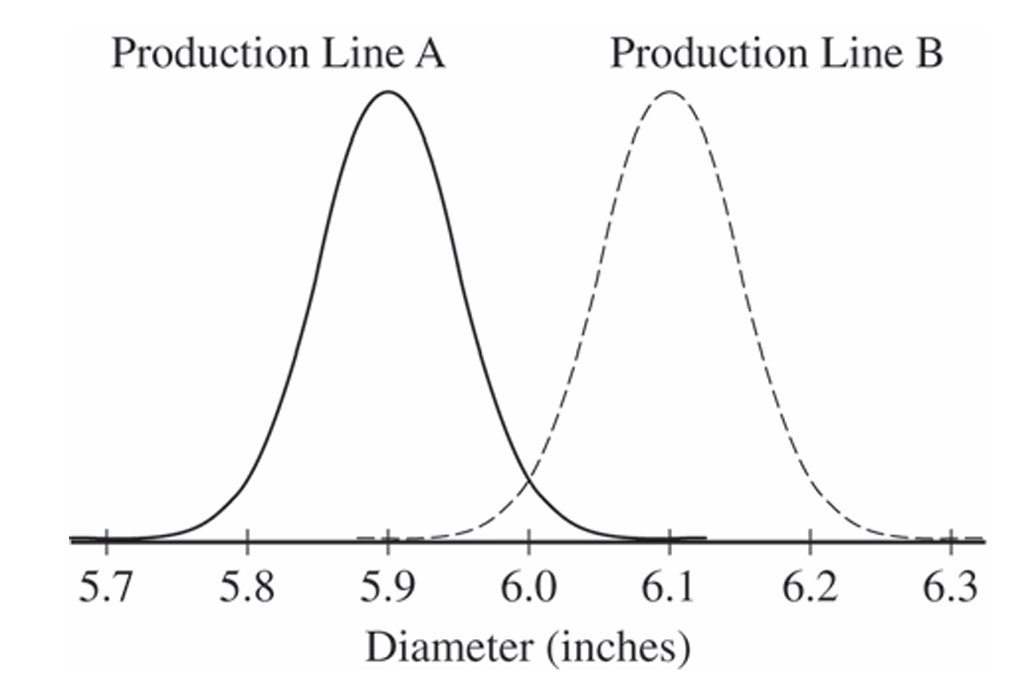
Corn tortillas are made at a large facility that produces $100,000$ tortillas per day on each of its two production lines. The distribution of the diameters of the tortillas produced on production line A is approximately normal with mean $5.9$ inches, and the distribution of the diameters of the tortillas produced on production line B is approximately normal with mean $6.1$ inches. The figure below shows the distributions of diameters for the two production lines.

The tortillas produced at the factory are advertised as having a diameter of $6$ inches. For the purpose of quality control, a sample of $200$ tortillas is selected and the diameters are measured. From the sample of $200$ tortillas, the manager of the facility wants to estimate the mean diameter, in inches, of the $200,000$ tortillas produced on a given day.

Two sampling methods have been proposed.

Method 1: Take a random sample of $200$ tortillas from the $200,000$ tortillas produced on a given day. Measure the diameter of each selected tortilla.

Method 2: Randomly select one of the two production lines on a given day. Take a random sample of $200$ tortillas from the $100,000$ tortillas produced by the selected production line. Measure the diameter of each selected tortilla.

(a) Will a sample obtained using Method 2 be representative of the population of all tortillas made that day, with respect to the diameters of the tortillas? Explain why or why not.

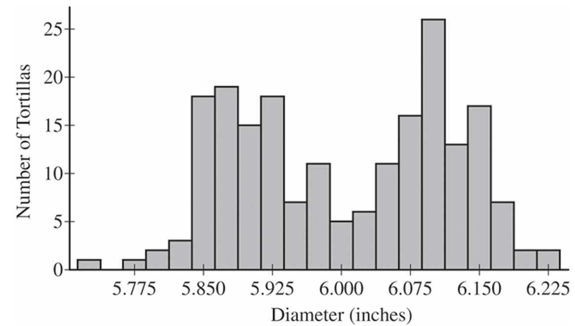
(b) The figure below is a histogram of $200$ diameters obtained by using one of the two sampling methods described. Considering the shape of the histogram, explain which method, Method 1 or Method 2, was most likely used to obtain a such a sample.

(c) Which of the two sampling methods, Method 1 or Method 2, will result in less variability in the diameters of the $200$ tortillas in the sample on a given day? Explain.

Each day, the distribution of the $200,000$ tortillas made that day has mean diameter $6$ inches with standard deviation $0.11$ inch.

(d) For samples of size $200$ taken from one day’s production, describe the sampling distribution of the sample mean diameter for samples that are obtained using Method 1.

(e) Suppose that one of the two sampling methods will be selected and used every day for one year ($365$ days). The sample mean of the $200$ diameters will be recorded each day. Which of the two methods will result in less variability in the distribution of the $365$ sample means? Explain.

(f) A government inspector will visit the facility on June $22$ to observe the sampling and to determine if the factory is in compliance with the advertised mean diameter of $6$ inches. The manager knows that, with both sampling methods, the sample mean is an unbiased estimator of the population mean. However, the manager is unsure which method is more likely to produce a sample mean that is close to $6$ inches on the day of sampling. Based on your previous answers, which of the two sampling methods, Method 1 or Method 2, is more likely to produce a sample mean close to $6$ inches? Explain.

Most-appropriate topic codes (AP Statistics):

• Topic $1.11$ — Random Samples and Simple Random Sampling (Parts $ \mathrm{a} $, $ \mathrm{b} $, $ \mathrm{c} $)
• Topic $4.1$ — Sampling Distributions for Sample Means (Parts $ \mathrm{d} $, $ \mathrm{e} $, $ \mathrm{f} $)

▶️ Answer/Explanation

(a)
No, a sample obtained using Method 2 will not be representative of all tortillas made that day. The sample obtained using Method 2 will only represent the tortillas from one production line, not from the entire population. Because the distributions of diameters for the two production lines are different, sampling from only one line misses the true characteristics of the combined production.

(b)
Method 1 was most likely used to select this sample. The bimodal shape in the histogram of sample data indicates that tortillas were selected from both production lines (with peaks around $5.9$ and $6.1$), which is what would happen using Method 1. Method 2 would be likely to produce a unimodal distribution centered at either $5.9$ inches or $6.1$ inches.

(c)
Method 2 would result in less variability in the sample of $200$ tortillas on a given day because the sample comes from only one production line. Since the distributions of diameters are not the same for the two production lines, selecting tortillas from both lines (as in Method 1) combines their differences and results in more variable sample data.

(d)
The sampling distribution of the sample mean diameter for samples obtained using Method 1 would be approximately normal because the sample size is large ($n = 200 \ge 30$), satisfying the Central Limit Theorem.

The mean of the sampling distribution is:
$ \mu_{\bar{x}} = \mu = 6 \text{ inches} $

The standard deviation (standard error) of the sampling distribution is:
$ \sigma_{\bar{x}} = \dfrac{\sigma}{\sqrt{n}} = \dfrac{0.11}{\sqrt{200}} \approx 0.0078 \text{ inch} $

(e)
Method 1 would result in less variability in the distribution of the $365$ sample means. The sample means from Method 1 will all be clustered very closely around the true population mean of $6$ inches. Conversely, the sample means from Method 2 will be clustered around $5.9$ inches on some days and around $6.1$ inches on other days, creating a much wider overall spread for the $365$ daily means.

(f)
Method 1 is more likely to produce a sample mean close to $6$ inches. Even though both methods are unbiased estimators in the long run, Method 1 consistently samples from the entire population and its sample mean has very little variability ($SE \approx 0.0078$). On the day of the inspection, Method 2 will likely produce a sample mean clustered near either $5.9$ inches or $6.1$ inches, which is relatively far from the advertised $6$ inches.

Question

Schools in a certain state receive funding based on the number of students who attend the school. To determine the number of students who attend a school, one school day is selected at random and the number of students in attendance that day is counted and used for funding purposes. The daily number of absences at High School A in the state is approximately normally distributed with mean of 120 students and standard deviation of 10.5 students.

(a) If more than 140 students are absent on the day the attendance count is taken for funding purposes, the school will lose some of its state funding in the subsequent year. Approximately what is the probability that High School A will lose some state funding?

(b) The principals’ association in the state suggests that instead of choosing one day at random, the state should choose 3 days at random. With the suggested plan, High School A would lose some of its state funding in the subsequent year if the mean number of students absent for the 3 days is greater than 140. Would High School A be more likely, less likely, or equally likely to lose funding using the suggested plan compared to the plan described in part (a)? Justify your choice.

(c) A typical school week consists of the days Monday, Tuesday, Wednesday, Thursday, and Friday. The principal at High School A believes that the number of absences tends to be greater on Mondays and Fridays, and there is concern that the school will lose state funding if the attendance count occurs on a Monday or Friday. If one school day is chosen at random from each of 3 typical school weeks, what is the probability that none of the 3 days chosen is a Tuesday, Wednesday, or Thursday?

Most-appropriate topic codes (AP Statistics):

• Topic $2.7$ — Normal Probability Distributions (Part $ \mathrm{a} $)
• Topic $4.1$ — Sampling Distributions for Sample Means (Part $ \mathrm{b} $)
• Topic $2.6$ — Probability Rules and Calculations of Probability (Part $ \mathrm{c} $)

▶️ Answer/Explanation

(a)
The daily number of absences follows an approximately normal distribution with $\mu = 120$ and $\sigma = 10.5$. We need $P(X > 140)$.
First, compute the $z$-score for $x = 140$:
$z = \dfrac{x – \mu}{\sigma} = \dfrac{140 – 120}{10.5} \approx 1.90$
From the standard normal table, $P(Z \leq 1.90) = 0.9713$, so:
$P(X > 140) = 1 – P(Z \leq 1.90) = 1 – 0.9713 = 0.0287$
$\boxed{P(\text{lose funding}) \approx 0.0287}$

(b)
High School A would be less likely to lose funding under the suggested plan.
Under the suggested plan, the relevant quantity is the sample mean $\bar{x}$ of absences over 3 days. By the Central Limit Theorem, $\bar{x}$ is approximately normally distributed with the same mean $\mu_{\bar{x}} = 120$ but a smaller standard deviation:
$\sigma_{\bar{x}} = \dfrac{\sigma}{\sqrt{n}} = \dfrac{10.5}{\sqrt{3}} \approx 6.062$
Now compute the $z$-score for $\bar{x} = 140$:
$z = \dfrac{140 – 120}{6.062} \approx 3.30$
From the standard normal table, $P(Z \leq 3.30) = 0.9995$, so:
$P(\bar{x} > 140) = 1 – 0.9995 = 0.0005$
Since $0.0005 < 0.0287$, the school is less likely to lose funding under the 3-day plan. Taking the average over multiple days reduces variability, making it much harder for the mean to stray as far as 140 from the center of 120.

(c)
A typical school week has 5 days: Monday, Tuesday, Wednesday, Thursday, and Friday. The “bad” days (Monday or Friday) number 2 out of 5, while the “safe” days (Tuesday, Wednesday, or Thursday) number 3 out of 5.
We want the probability that none of the 3 days chosen (one from each of 3 weeks) is a Tuesday, Wednesday, or Thursday — meaning all 3 days must be Monday or Friday.
For any one week, the probability of choosing a Monday or Friday is:
$P(\text{Mon or Fri}) = \dfrac{2}{5} = 0.4$
Since the day chosen each week is independent of the other weeks:
$P(\text{none of the 3 days is Tue, Wed, or Thu}) = (0.4)^3 = 0.064$
$\boxed{P = 0.064}$

Question

Two students at a large high school, Peter and Rania, wanted to estimate $\mu$, the mean number of soft drinks that a student at their school consumes in a week. A complete roster of the names and genders for the 2,000 students at their school was available. Peter selected a simple random sample of 100 students. Rania, knowing that 60 percent of the students at the school are female, selected a simple random sample of 60 females and an independent simple random sample of 40 males. Both asked all of the students in their samples how many soft drinks they typically consume in a week.

(a) Describe a method Peter could have used to select a simple random sample of 100 students from the school.

Peter and Rania conducted their studies as described. Peter used the sample mean $\bar{X}$ as a point estimator for $\mu$. Rania used $\bar{X}_{strat} = 0.6\bar{X}_{female} + 0.4\bar{X}_{male}$ as a point estimator for $\mu$, where $\bar{X}_{female}$ is the mean of the sample of 60 females and $\bar{X}_{male}$ is the mean of the sample of 40 males.

Summary statistics for Peter’s data are shown in the table below.

(b) Based on the summary statistics, calculate the estimated standard deviation of the sampling distribution (sometimes called the standard error) of Peter’s point estimator $\bar{X}$.

Summary statistics for Rania’s data are shown in the table below.

(c) Based on the summary statistics, calculate the estimated standard deviation of the sampling distribution of Rania’s point estimator $\bar{X}_{strat}$.

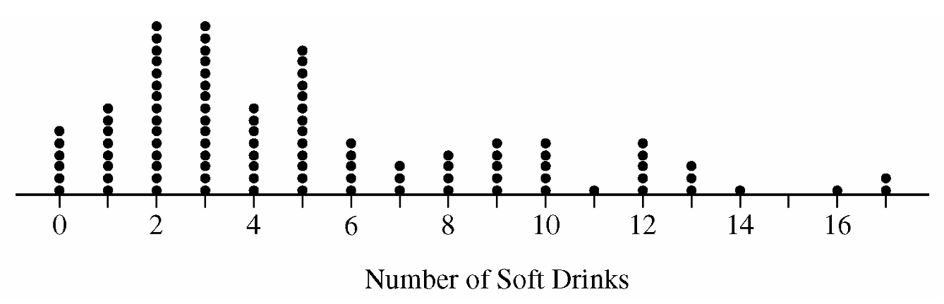
A dotplot of Peter’s sample data is given below.

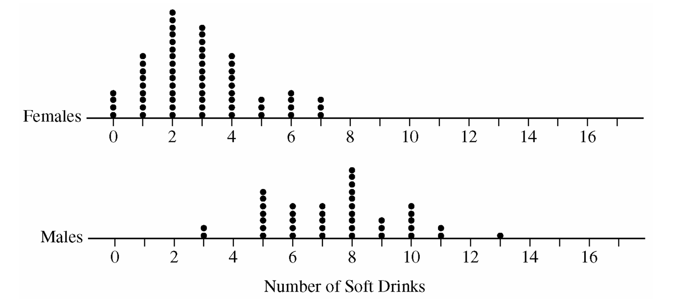
Comparative dotplots of Rania’s sample data are given below.

(d) Using the dotplots above, explain why Rania’s point estimator has a smaller estimated standard deviation than the estimated standard deviation of Peter’s point estimator.

Most-appropriate topic codes (AP Statistics):

• Topic 1.11 — Random Sampling (Part a)
• Topic 4.1 — Sampling Distributions for Sample Means (Parts b, c)
• Topic 4.1 — Sampling Distributions for Sample Means (Part d)
• Topic 1.11 — Random Sampling (Part d)

▶️ Answer/Explanation

(a)
To select a proper simple random sample, Peter could number all the students on the roster from 1 to 2,000.
Then, he can use a random number generator to produce numbers between 1 and 2,000.
He would ignore any repeated numbers and continue generating until he has a list of 100 unique random numbers.
The 100 students corresponding to those selected numbers will make up his sample.

(b)
The estimated standard deviation of the sampling distribution of the sample mean (standard error) for Peter’s simple random sample is calculated using the formula $\text{SE}(\bar{X}) = \frac{s}{\sqrt{n}}$.
Substituting the values from Peter’s sample: $\text{SE}(\bar{X}) = \frac{4.13}{\sqrt{100}}$.
$\text{SE}(\bar{X}) = \frac{4.13}{10} = 0.413$.
The estimated standard deviation of Peter’s point estimator is $0.413$.

(c)
Rania’s point estimator is given by $\bar{X}_{strat} = 0.6\bar{X}_{female} + 0.4\bar{X}_{male}$.
Because the two samples (female and male) are independent, the variance of the stratified estimator is the sum of the variances of each part, scaled by their squared weights:
$\text{Var}(\bar{X}_{strat}) = (0.6)^2 \text{Var}(\bar{X}_{female}) + (0.4)^2 \text{Var}(\bar{X}_{male})$.
The variance for the female sample mean is $\frac{s_{f}^2}{n_f} = \frac{(1.80)^2}{60} = \frac{3.24}{60} = 0.054$.
The variance for the male sample mean is $\frac{s_{m}^2}{n_m} = \frac{(2.22)^2}{40} = \frac{4.9284}{40} = 0.12321$.
Substitute these into the combined variance equation:
$\text{Var}(\bar{X}_{strat}) = (0.36)(0.054) + (0.16)(0.12321) = 0.01944 + 0.0197136 = 0.0391536$.
The estimated standard deviation is the square root of the variance:
$\text{SE}(\bar{X}_{strat}) = \sqrt{0.0391536} \approx 0.198$.

(d)
Based on the dotplots, there is a clear difference in the soft drink consumption patterns between genders. The dotplot for males indicates a visibly higher center (around 7-8 drinks) compared to the dotplot for females (centered around 2-3 drinks).
Because of this distinct separation between the two groups, a standard simple random sample like Peter’s will experience a large amount of variation as different samples will randomly capture varying proportions of males and females, producing a wider overall spread (standard deviation of 4.13).
By contrast, Rania’s stratified method guarantees that the sample consists of exactly 60% females and 40% males. The variability within each homogeneous gender group (1.80 for females and 2.22 for males) is much smaller than the overall variability of the mixed population.
Because stratification eliminates the between-group variation from the standard error calculation, Rania’s point estimator results in a substantially smaller estimated standard deviation.

Question

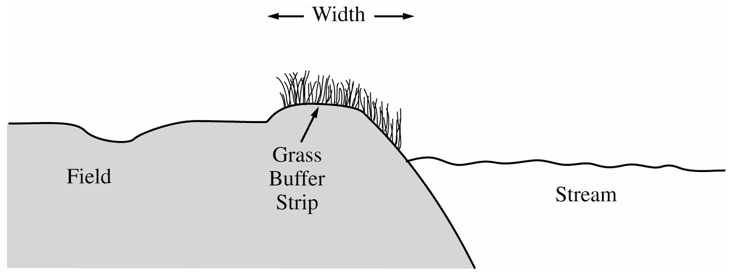
Grass buffer strips are grassy areas that are planted between bodies of water and agricultural fields. These strips are designed to filter out sediment, organic material, nutrients, and chemicals carried in runoff water. The figure below shows a cross-sectional view of a grass buffer strip that has been planted along the side of a stream.

A study in Nebraska investigated the use of buffer strips of several widths between 5 feet and 15 feet. The study results indicated a linear relationship between the width of the grass strip ($x$), in feet, and the amount of nitrogen removed from the runoff water ($y$), in parts per hundred. The following model was estimated.

$\hat{y} = 33.8 + 3.6x$

(a) Interpret the slope of the regression line in the context of this question.

(b) Would you be willing to use this model to predict the amount of nitrogen removed for grass buffer strips with widths between 0 feet and 30 feet? Explain why or why not.

A scientist in California wants to know if there is a similar relationship in her area. To investigate this, she will place a grass buffer strip between a field and a nearby stream at each of eight different locations and measure the amount of nitrogen that the grass buffer strip removes, in parts per hundred, from runoff water at each location. Each of the eight locations can accommodate a buffer strip between 6 feet and 13 feet in width. The scientist wants to investigate which combination of widths will provide the best estimate of the slope of the regression line.

Suppose the scientist decides to use buffer strips of width 6 feet at each of four locations and buffer strips of width 13 feet at each of the other four locations. Assume the model, $\hat{y} = 33.8 + 3.6x$, estimated from the Nebraska study is the true regression line in California and the observations at the different locations are normally distributed with standard deviation of 5 parts per hundred.

(c) Describe the sampling distribution of the sample mean of the observations on the amount of nitrogen removed by the four buffer strips with widths of 6 feet.

(d) Using your result from part (c), show how to construct an interval that has probability 0.95 of containing the sample mean of the observations from four buffer strips with widths of 6 feet.

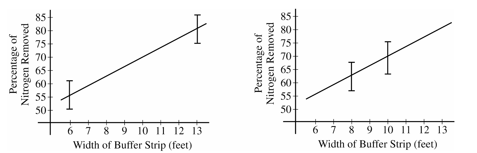
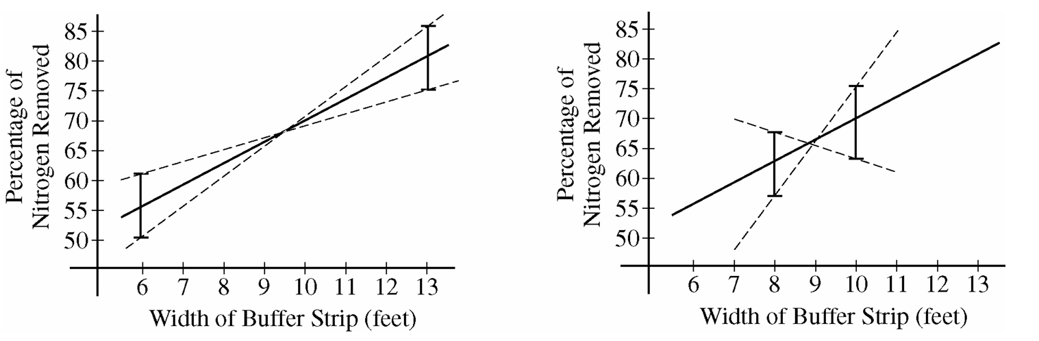
For the study plan being implemented by the scientist in California, the graph on the left below displays intervals that each have probability 0.95 of containing the sample mean of the four observations for buffer strips of width 6 feet and for buffer strips of width 13 feet. A second possible study plan would use buffer strips of width 8 feet at four of the eight locations and buffer strips of width 10 feet at the other four locations. Intervals that each have probability 0.95 of containing the mean of the four observations for buffer strips of width 8 feet and for buffer strips of width 10 feet, respectively, are shown in the graph on the right below.

If data are collected for the first study plan, a sample mean will be computed for the four observations from buffer strips of width 6 feet and a second sample mean will be computed for the four observations from buffer strips of width 13 feet. The estimated regression line for those eight observations will pass through the two sample means. If data are collected for the second study plan, a similar method will be used.

(e) Use the plots above to determine which study plan, the first or the second, would provide a better estimator of the slope of the regression line. Explain your reasoning.

(f) The previous parts of this question used the assumption of a straight-line relationship between the width of the buffer strip and the amount of nitrogen that is removed, in parts per hundred. Although this assumption was motivated by prior experience, it may not be correct. Describe another way of choosing the widths of the buffer strips at eight locations that would enable the researchers to check the assumption of a straight-line relationship.

Most-appropriate topic codes (AP Statistics):

• Topic 5.3 — Linear Regression Models (Parts a, b)
• Topic 4.1 — Sampling Distributions for Sample Means (Parts c, d)
• Topic 5.5 — Least-Squares Regression (Part e)
• Topic 1.13 — Experimental Design (Part f)

▶️ Answer/Explanation

(a)

The slope of the regression line is $3.6$.

This means that for each additional foot added to the width of the grass buffer strip, the amount of nitrogen removed from the runoff water increases by approximately $3.6$ parts per hundred, on average.

(b)

No — this model should not be used for widths between 0 and 30 feet.

The Nebraska study only investigated buffer strips with widths between 5 feet and 15 feet, so the linear relationship was established only within that range.

Predicting for widths as small as 0 feet or as large as 30 feet would be extrapolation far beyond the data, making such predictions unreliable and potentially meaningless.

(c)

When the buffer strip width is $x = 6$ feet, the true mean nitrogen removed is predicted by the model as:

$\mu = 33.8 + 3.6(6) = 33.8 + 21.6 = 55.4 \text{ parts per hundred}$

Since individual observations are normally distributed with standard deviation $\sigma = 5$, the sampling distribution of the sample mean $\bar{x}$ of four observations is normal with:

$\mu_{\bar{x}} = 55.4 \text{ parts per hundred}$

$\sigma_{\bar{x}} = \frac{\sigma}{\sqrt{n}} = \frac{5}{\sqrt{4}} = 2.5 \text{ parts per hundred}$

So the sampling distribution is $N(55.4,\ 2.5)$.

(d)

Since the sampling distribution of $\bar{x}$ is normal, use the critical value $z^* = 1.96$ for a probability of 0.95.

The interval is constructed as:

$\mu_{\bar{x}} \pm z^* \cdot \sigma_{\bar{x}} = 55.4 \pm 1.96 \times 2.5 = 55.4 \pm 4.9$

$\Rightarrow \left(55.4 – 4.9,\ \ 55.4 + 4.9\right) = (50.5,\ \ 60.3)$

There is probability 0.95 that the sample mean of four 6-foot buffer strip observations falls between $50.5$ and $60.3$ parts per hundred.

(e)

The first study plan (widths 6 feet and 13 feet) provides the better estimator of the slope.

The estimated regression line must pass through the two sample means, so any variation in those sample means produces variation in the estimated slope.

In Study Plan 1, the two $x$-values ($6$ ft and $13$ ft) are spread far apart; even with vertical spread in the 0.95-probability intervals, the range of possible connecting slopes is relatively narrow — as seen in the left graph.

In Study Plan 2, the two $x$-values ($8$ ft and $10$ ft) are close together; the same vertical spread in the intervals produces a much wider range of possible slopes — as seen in the right graph.

Therefore, the sampling variability of the estimated slope $\hat{b}$ is smaller under Study Plan 1, making it the better estimator of the true slope.

(f)

To check the linearity assumption, the researcher should use buffer strips of more than two different widths spread across the entire range of interest (6 to 13 feet).

For example, she could use eight different widths — one at each location — such as 6, 7, 8, 9, 10, 11, 12, and 13 feet.

With data at many distinct widths, a scatterplot of nitrogen removed versus strip width would reveal whether the relationship follows a straight line or shows curvature, directly allowing the researchers to assess the straight-line assumption.

Question

A local news channel monitors the length of time of each song played by a popular satellite radio station. A random sample of 40 songs played by the station was selected, and the length of each song was recorded. The mean length of the 40 songs was 3.9 minutes with a standard deviation of 1.1 minutes. The distribution of song lengths in the population is known to be roughly symmetric, but not normal.

(a) Describe the sampling distribution of the sample mean song length for random samples of 40 songs from this station.

(b) The satellite radio station has 4 hours (240 minutes) of commercial-free airtime each night. If 40 songs are randomly selected and played commercial-free, what is the probability that the total airtime required to play the 40 songs exceeds the available 4 hours?

Most-appropriate topic codes (AP Statistics):

• Topic 4.1 — Sampling Distributions for Sample Means (Part a)
• Topic 2.12 — Sampling Distributions and the Central Limit Theorem (Part a)
• Topic 4.1 — Sampling Distributions for Sample Means (Part b)

▶️ Answer/Explanation

(a)

The sampling distribution of the sample mean song length $\overline{X}$ can be described completely by three attributes:
Center: The mean of the sampling distribution is equal to the population mean, so $\mu_{\overline{X}} = \mu = 3.9\text{ minutes}$.
Spread: The standard deviation of the sampling distribution is computed using the population standard deviation divided by the square root of the sample size:
$\sigma_{\overline{X}} = \dfrac{\sigma}{\sqrt{n}} = \dfrac{1.1}{\sqrt{40}} \approx 0.174\text{ minutes}$
Shape: Since the sample size $n = 40$ is sufficiently large ($n \ge 30$), the Central Limit Theorem applies directly. Even though the original population distribution is non-normal, the shape of the sampling distribution of the sample mean will be approximately normal.

(b)

The probability that the total airtime of 40 randomly selected songs exceeds the available time (that is, the probability that the total airtime of 40 randomly selected songs is greater than 160 minutes) is equivalent to the probability that the sample mean length of the 40 songs is greater than $\dfrac{160}{40} = 4.0$ minutes.
According to part (a), the distribution of the sample mean length $\overline{X}$ is approximately normal. Therefore,
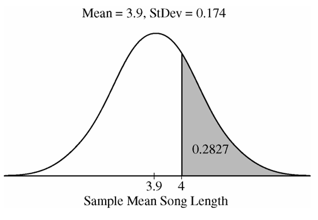
$P(\overline{X} > 4.0) \approx P\left( Z > \dfrac{4.0 – 3.9}{0.174} \right) = P(Z > 0.57) = 1 – 0.7157 = 0.2843$.
(The calculator gives the answer as 0.2827.)
The approximate sampling distribution of the sample mean song length and the desired probability are displayed below.

Question

A car manufacturer is interested in conducting a study to estimate the mean stopping distance for a new type of brakes when used in a car that is traveling at 60 miles per hour. These new brakes will be installed on cars of the same model and the stopping distance will be observed. The cost of each observation is $\$100$. A budget of $\$12{,}000$ is available to conduct the study and the goal is to carry it out in the most economical way possible. Preliminary studies indicate that $\sigma = 12$ feet for stopping distances.

(a) Are sufficient funds available to estimate the mean stopping distance to within $2$ feet of the true mean stopping distance with $95\%$ confidence?

Explain your answer.

(b) A regulatory agency requires a $95\%$ level of confidence for an estimate of mean stopping distance that is within $2$ feet of the true mean stopping distance. The car manufacturer cannot exceed the budget of $\$12{,}000$ for the study. Discuss the consequences of these constraints.

Most-appropriate topic codes (AP Statistics):

• Topic 4.2 — Constructing a Confidence Interval for a Population Mean or Population Mean Difference (Parts $\mathrm{a}$, $\mathrm{b}$)
• Topic 4.1 — Sampling Distributions for Sample Means (Part $\mathrm{a}$)

▶️ Answer/Explanation

(a)
No, sufficient funds are not available.
To estimate the mean to within a margin of error $E = 2$ feet with $95\%$ confidence, we use the sample size formula:
$n = \left(\frac{z^* \cdot \sigma}{E}\right)^2$
With $z^* = 1.96$, $\sigma = 12$, and $E = 2$:
$n = \left(\frac{1.96 \times 12}{2}\right)^2 = \left(\frac{23.52}{2}\right)^2 = (11.76)^2 = 138.3$
Since sample size must be a whole number, we round up:
$\boxed{n = 139}$
The cost of conducting 139 observations would be:
$139 \times \$100 = \$13{,}900$
Since $\$13{,}900 > \$12{,}000$, the budget is insufficient to achieve the desired margin of error.
Alternatively, with a budget of $\$12{,}000$, the manufacturer can afford at most:
$n = \frac{\$12{,}000}{\$100} = 120 \text{ observations}$
The margin of error achievable with $n = 120$ is:
$E = 1.96 \times \frac{12}{\sqrt{120}} = 1.96 \times 1.095 \approx 2.15 \text{ feet}$
Since $2.15 > 2$, the required precision of $2$ feet cannot be met with the available budget.
$\boxed{\text{Sufficient funds are NOT available}}$

(b)
The two constraints — a $95\%$ confidence level with a margin of error within $2$ feet, and a budget cap of $\$12{,}000$ — are in direct conflict with each other.
Meeting the regulatory agency’s requirement demands at least $139$ observations, which costs $\$13{,}900$. The budget of $\$12{,}000$ only allows $120$ observations, which yields a margin of error of approximately $2.15$ feet at the $95\%$ confidence level.
Since $2.15 > 2$, the manufacturer cannot simultaneously satisfy both the statistical requirement (within $2$ feet) and the financial constraint ($\$12{,}000$ budget).
As a consequence, the car manufacturer will not be able to meet the regulatory agency’s requirements with the allocated budget. Unless the budget is increased to at least $\$13{,}900$, or the agency relaxes its precision requirement, the manufacturer cannot obtain regulatory approval under the current constraints.
$\boxed{\text{The manufacturer cannot meet the regulatory requirement within the given budget}}$

Question

Big Town Fisheries recently stocked a new lake in a city park with 2,000 fish of various sizes. The distribution of the lengths of these fish is approximately normal.

(a) Big Town Fisheries claims that the mean length of the fish is 8 inches. If the claim is true, which of the following would be more likely?

• A random sample of 15 fish having a mean length that is greater than 10 inches

• A random sample of 50 fish having a mean length that is greater than 10 inches

Justify your answer.

(b) Suppose the standard deviation of the sampling distribution of the sample mean for random samples of size 50 is 0.3 inch. If the mean length of the fish is 8 inches, use the normal distribution to compute the probability that a random sample of 50 fish will have a mean length less than 7.5 inches.

(c) Suppose the distribution of fish lengths in this lake was nonnormal but had the same mean and standard deviation. Would it still be appropriate to use the normal distribution to compute the probability in part (b)? Justify your answer.

Most-appropriate topic codes (AP Statistics):

• Topic 2.12 — Sampling Distributions and the Central Limit Theorem (Parts $\mathrm{a}$, $\mathrm{c}$)
• Topic 4.1 — Sampling Distributions for Sample Means (Part $\mathrm{a}$)
• Topic 2.11 — The Normal Distribution (Part $\mathrm{b}$)

▶️ Answer/Explanation

(a)

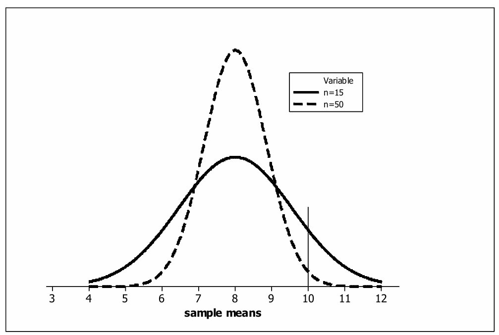
A random sample of $n = 15$ fish is more likely to have a sample mean greater than 10 inches.
Both sampling distributions are centered at the true mean $\mu = 8$ inches, but they differ in their variability. The standard deviation of the sampling distribution of the sample mean is given by $\dfrac{\sigma}{\sqrt{n}}$, so a smaller sample size produces a larger standard deviation — meaning the distribution is more spread out.
Since the sampling distribution for $n = 15$ is more spread out than for $n = 50$, the tail area beyond 10 inches is larger for $n = 15$, making it more likely to observe a sample mean greater than 10 inches with the smaller sample.
$\boxed{P(\bar{x} > 10 \mid n=15) > P(\bar{x} > 10 \mid n=50) \text{ because the } n=15 \text{ distribution has greater variability.}}$

(b)

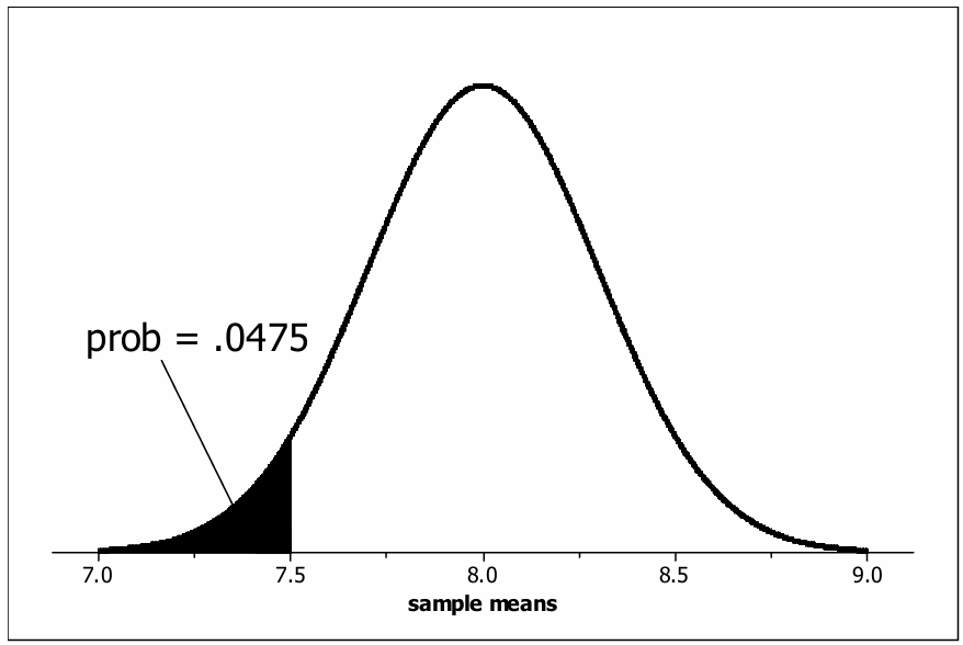
We are given: $\mu = 8$, $\sigma_{\bar{x}} = 0.3$, and we want $P(\bar{x} < 7.5)$.
First, compute the $z$-score:
$z = \dfrac{\bar{x} – \mu}{\sigma_{\bar{x}}} = \dfrac{7.5 – 8}{0.3} = \dfrac{-0.5}{0.3} \approx -1.67$
Now look up the standard normal table for $z = -1.67$:
$P(\bar{x} < 7.5) = P(z < -1.67) \approx 0.0475$
$\boxed{P(\bar{x} < 7.5) \approx 0.0475}$

(c)

Yes, it would still be appropriate to use the normal distribution to compute this probability.
By the Central Limit Theorem (CLT), the sampling distribution of the sample mean $\bar{x}$ is approximately normal for sufficiently large sample sizes, regardless of the shape of the population distribution.
Since our sample size is $n = 50$, which is reasonably large (generally $n \geq 30$ is considered sufficient), the CLT guarantees that $\bar{x}$ follows an approximately normal distribution even if the individual fish lengths are nonnormally distributed.
Therefore, the probability calculated in part (b) remains a good approximation.
$\boxed{\text{Yes — by the CLT, } n = 50 \text{ is large enough for the sampling distribution of } \bar{x} \text{ to be approximately normal.}}$

Question

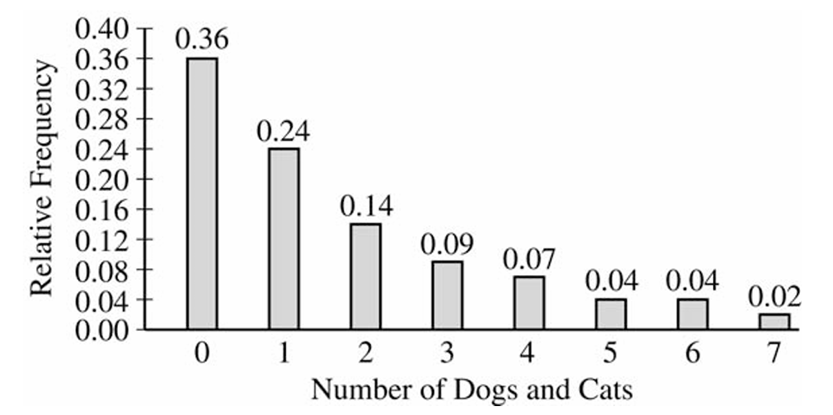
The graph below displays the relative frequency distribution for $X$, the total number of dogs and cats owned per household, for the households in a large suburban area. For instance, $14$ percent of the households own $2$ of these pets.

(a) According to a local law, each household in this area is prohibited from owning more than $3$ of these pets. If a household in this area is selected at random, what is the probability that the selected household will be in violation of this law? Show your work.

(b) If $10$ households in this area are selected at random, what is the probability that exactly $2$ of them will be in violation of this law? Show your work.

(c) The mean and standard deviation of $X$ are $1.65$ and $1.851$, respectively. Suppose $150$ households in this area are to be selected at random and $\bar{X}$, the mean number of dogs and cats per household, is to be computed. Describe the sampling distribution of $\bar{X}$, including its shape, center, and spread.

Most-appropriate topic codes (AP Statistics):

• Topic 2.4 — Introduction to Probability (Part $\mathrm{a}$)
• Topic 2.10 — The Binomial Distribution (Part $\mathrm{b}$)
• Topic 2.8 — Introduction to Random Variables and Probability Distributions (Parts $\mathrm{a}$, $\mathrm{b}$)
• Topic 2.12 — Sampling Distributions and the Central Limit Theorem (Part $\mathrm{c}$)
• Topic 4.1 — Sampling Distributions for Sample Means (Part $\mathrm{c}$)

▶️ Answer/Explanation

(a)
A household is in violation if it owns more than $3$ pets, i.e., $X > 3$. Read the relative frequencies for $X = 4, 5, 6, 7$ directly from the graph and add them up.
$P(X > 3) = P(X=4) + P(X=5) + P(X=6) + P(X=7)$
$P(X > 3) = 0.07 + 0.04 + 0.04 + 0.02$
$\boxed{P(X > 3) = 0.17}$

(b)
Let $Y$ = the number of households in violation among the $10$ selected. Since each household is independently either in violation or not, $Y$ follows a binomial distribution with $n = 10$ and $p = 0.17$ (from part (a)).
Using the binomial probability formula $P(Y = k) = \dbinom{n}{k} p^k (1-p)^{n-k}$:
$P(Y = 2) = \binom{10}{2}(0.17)^2(0.83)^8$
$P(Y = 2) = 45 \times (0.0289) \times (0.2252)$
$\boxed{P(Y = 2) \approx 0.2929}$

(c)
Because the sample size $n = 150$ is large, the Central Limit Theorem tells us the sampling distribution of $\bar{X}$ will be approximately normal, regardless of the shape of the original population distribution.
The mean of the sampling distribution equals the population mean:
$\mu_{\bar{X}} = \mu = 1.65$
The standard deviation (standard error) of the sampling distribution is:
$\sigma_{\bar{X}} = \dfrac{\sigma}{\sqrt{n}} = \dfrac{1.851}{\sqrt{150}} \approx 0.1511$
So the sampling distribution of $\bar{X}$ is approximately $N(1.65,\ 0.1511)$ — normal, centered at $1.65$, with a standard deviation of about $0.1511$.

AP Statistics 4.1 Sampling Distributions for Sample Means- Exam Style Questions - FRQs - New Syllabus

Question

Question

Question

Question

Question

Question

Question

Question

Resources

Members

Company