AP Statistics 4.10 Carrying Out a Test for the Difference Between Two Population Means- Exam Style Questions - FRQs - New Syllabus

Question

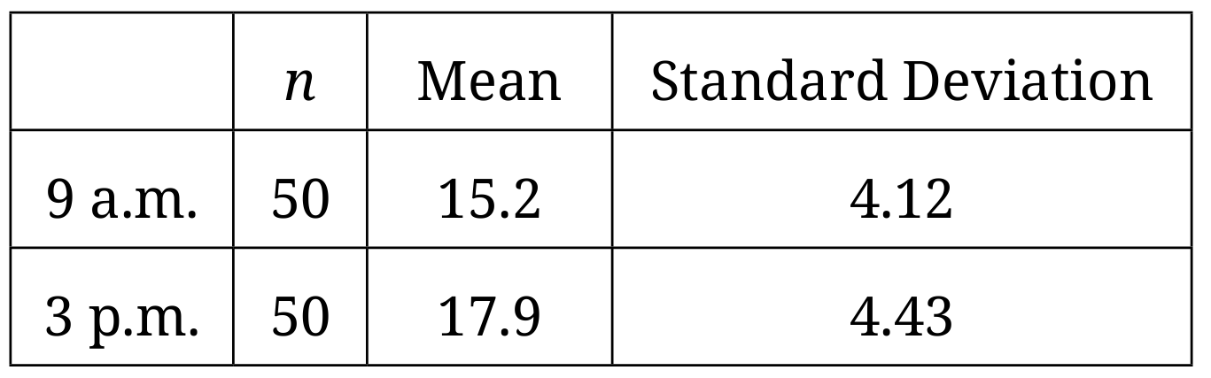
Stefan, a psychologist, conducted a study to investigate the effect of time of day on reading comprehension in children. One hundred children volunteered, with their parents’ consent, to participate in the study. Fifty of the children were randomly assigned to read a story at 9 a.m. and then answer 25 questions about it. The remaining 50 children were assigned to read the same story at 3 p.m. and answer the same 25 questions. The reading comprehension for each child was measured by a reading score, which was determined by the number of questions that were answered correctly about the story. Stefan is interested in comparing the mean reading scores for the two times of day. Table 1 shows the results of Stefan’s study.

Table 1: Summary Statistics of Reading Scores

Stefan found the conditions for inference were met and conducted a two-sample t-test for the difference in two population means. Let $\mu_{\text{AM}}$ represent the mean reading score for all children, similar to those in the study, who would read the story at 9 a.m. Let $\mu_{\text{PM}}$ represent the mean reading score for all children, similar to those in the study, who would read the story at 3 p.m. Stefan’s hypotheses are as shown.

$H_0: \mu_{\text{AM}} = \mu_{\text{PM}}$
$H_a: \mu_{\text{AM}} \neq \mu_{\text{PM}}$

A. The p-value for Stefan’s hypothesis test was 0.002. State an appropriate conclusion, at the 5 percent significance level, for Stefan’s test in the context of the investigation. Justify your answer.

B. Explain why it was appropriate for Stefan to conduct a two-sample t-test for the difference in two population means instead of a paired t-test for the population mean difference.

C. Researchers are usually interested in the practical importance of their results as well as the statistical significance of the hypothesis test. The practical importance of the results indicates whether the observed results are meaningful in real life. For example, in an investigation of the heights of two groups of students, a difference in the two group means of 3.8 inches is much more meaningful, or has more practical importance, than a difference in the two group means of only 0.2 inches.

One indicator of practical importance is effect size. A common method for measuring effect size for the difference in two group means is Cohen’s d coefficient. Cohen’s d coefficient compares the absolute value of the difference in the means of the two groups to the pooled variability of the observed data values from the two groups. Cohen’s d coefficient can be calculated using

$d = \dfrac{|\bar{x}_1 – \bar{x}_2|}{s_p}$

where $s_p$ represents the pooled standard deviation, $\bar{x}_1$ represents the sample mean for the first group, and $\bar{x}_2$ represents the sample mean for the second group. When the sizes of the groups are equal, $s_p$ is calculated as

$s_p = \sqrt{\dfrac{s_1^2 + s_2^2}{2}}$

where $s_1$ represents the sample standard deviation for the first group and $s_2$ represents the sample standard deviation for the second group. Consider the summary statistics from Stefan’s study in Table 1.

i. Calculate Cohen’s d coefficient for Stefan’s study. Show your work.
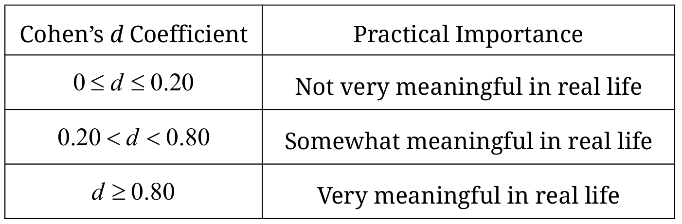
ii. Higher values of Cohen’s d indicate greater practical importance and lower values of Cohen’s d indicate less practical importance. Typically, we use the intervals listed in Table 2 to help interpret practical importance.

Table 2: Guidelines for Interpreting Cohen’s d Coefficient

Based on your answer to part C (i) and the information in Tables 1 and 2, describe the practical importance of Stefan’s results, in context.

D. Suppose the results of Stefan’s study, summarized in Table 1, instead had a standard deviation for the 9 a.m. reading scores, $s_1$, and a standard deviation for the 3 p.m. reading scores, $s_2$, that were both greater than 4.43. Assume the group sample sizes and the means are not changed.

i. Would the Cohen’s d coefficient in this new situation be smaller than, larger than, or the same as the Cohen’s d coefficient calculated in part C (i)? Explain your answer.
ii. Does the Cohen’s d coefficient described in part D (i) indicate that Stefan’s observed difference in the means in the new situation would have more practical importance than, less practical importance than, or the same practical importance as what was originally determined in part C (ii)? Explain your answer.

Most-appropriate topic codes (AP Statistics):

• Topic $4.9$ — Setting Up a Test for the Difference Between Two Population Means (Part $ \mathrm{B} $)
• Topic $4.10$ — Carrying Out a Test for the Difference Between Two Population Means (Parts $ \mathrm{A} $, $ \mathrm{C} $, $ \mathrm{D} $)

▶️ Answer/Explanation

A.
• Because the reported $p$-value ($0.002$) is less than the significance level $\alpha = 0.05$, we reject the null hypothesis $H_0$.
• There is convincing statistical evidence to conclude that there is a difference between the mean reading scores for all children, similar to those in the study, who read the story at 9 a.m. versus those who read at 3 p.m.

B.
• A two-sample $t$-test is appropriate here because the two groups of children are completely independent of each other rather than paired.
• The 100 individual volunteers were randomly split into separate blocks of 50, meaning there is no logical connection or unique pairing linking a specific child’s performance in the morning slot directly to another child’s performance in the afternoon slot.

C. i.
First compute the pooled standard deviation $s_p$:
$s_p = \sqrt{\dfrac{(4.12)^2 + (4.43)^2}{2}} = \sqrt{\dfrac{16.9744 + 19.6249}{2}} = \sqrt{\dfrac{36.5993}{2}} = \sqrt{18.29965} \approx 4.2778$
Now calculate the effect size $d$:
$d = \dfrac{|15.2 – 17.9|}{4.2778} = \dfrac{2.7}{4.2778} \approx 0.6311$
$\boxed{d \approx 0.63}$

C. ii.
• Based on the calculated Cohen’s $d$ value of $0.63$, which falls within the interval $(0.20, 0.80)$, the effect is classified as “somewhat meaningful in real life.”
• This indicates that the shift in mean reading performance across different times of the day is large enough to show noticeable practical consequences for children’s learning schedules, though it is not a overwhelmingly massive real-world shift.

D. i.
• The Cohen’s $d$ coefficient in this new scenario would be smaller than the value calculated originally.
• Since the separate group sample variations are now both larger than $4.43$, the pooled denominator value $s_p$ will increase, which reduces the final value of the quotient since the raw difference in means remains fixed at $2.7$.

D. ii.
• This modified index indicates that Stefan’s observed score gap would have less practical importance than what was originally determined.
• When individual scores overlap more heavily due to wider personal variation within each testing window, a constant mean gap of $2.7$ points becomes harder to detect cleanly and feels less distinct in practical environments.

Question

High cholesterol levels in people can be reduced by exercise, diet, and medication. Twenty male patients at a local hospital who had high cholesterol levels volunteered to participate in a simulated study. Ten of the twenty patients were randomly assigned to receive drug A, and the remaining ten patients received a placebo. Data on cholesterol reduction, in milligrams per deciliter (mg/dL), were recorded for the twenty patients twice: once after a 4-week period and again after an 8-week period. The results are summarized in the table below.

Do the data provide convincing statistical evidence that, at the $\alpha = 0.01$ level, the mean cholesterol reduction for all male patients who take drug A for 8 weeks is greater than the mean cholesterol reduction for all male patients who take a placebo for 8 weeks?

Most-appropriate topic codes (AP Statistics):

• Topic 4.9 — Setting Up a Test for the Difference Between Two Population Means (Entire Question)
• Topic 4.10 — Carrying Out a Test for the Difference Between Two Population Means (Entire Question)

▶️ Answer/Explanation

Step 1: State Hypotheses and Define Parameters
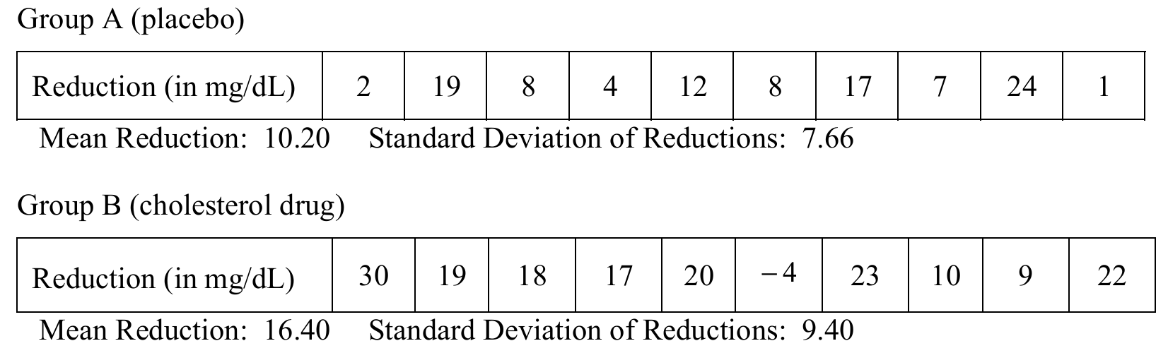
Let $\mu_{A}$ represent the true mean cholesterol reduction if all such male patients at this hospital receive Drug A for 8 weeks.
Let $\mu_{B}$ represent the true mean cholesterol reduction if all such male patients at this hospital receive a placebo for 8 weeks.
The hypotheses to be tested are:
$H_{0}: \mu_{A} = \mu_{B}$ (or $\mu_{A} – \mu_{B} = 0$)
$H_{a}: \mu_{A} > \mu_{B}$ (or $\mu_{A} – \mu_{B} > 0$)

Step 2: Identify the Procedure and Check Conditions

The appropriate method is a two-sample $t$-test for the difference between two population means.
• Random Assignment: The problem states that the 20 volunteers were randomly assigned to the treatment groups (10 to Group A and 10 to Group B).
• Normality: Because the sample sizes are quite small ($n_A = 10$ and $n_B = 10$), we must assume that the populations of cholesterol reductions are approximately normally distributed or that the sample data show no extreme outliers or strong skewness.

Step 3: Compute Test Statistic and $p$-value
Demonstrates correct mechanics, including the value of the test statistic and $p$-value (or the rejection region).
The test statistic is: $t = \dfrac{\bar{X}_A – \bar{X}_B}{\sqrt{\dfrac{s_A^2}{n_A} + \dfrac{s_B^2}{n_B}}} = \dfrac{10.20 – 16.40}{\sqrt{\dfrac{7.66^2}{10} + \dfrac{9.40^2}{10}}} \approx -1.62$
With $\text{df} = 17.3$, $p$-value $\approx 0.062$.

Step 4: Make a Conclusion
Since the $p$-value ($0.033$) is greater than the specified significance level $\alpha = 0.01$, we fail to reject the null hypothesis $H_{0}$.
The observed difference in mean cholesterol reduction between the two groups is not statistically large enough to rule out random chance at this strict standard. Consequently, the study does not provide convincing clinical evidence that the mean cholesterol reduction is greater for those taking Drug A for 8 weeks compared to those taking a placebo.

Question

A large pet store buys the identical species of adult tropical fish from two different suppliers—Buy-Rite Pets and Fish Friends. Several of the managers at the pet store suspect that the lengths of the fish from Fish Friends are consistently greater than the lengths of the fish from Buy-Rite Pets. Random samples of 8 adult fish of the species from Buy-Rite Pets and 10 adult fish of the same species from Fish Friends were selected and the lengths of the fish, in inches, were recorded, as shown in the table below.

Do the data provide convincing evidence that the mean length of the adult fish of the species from Fish Friends is greater than the mean length of the adult fish of the same species from Buy-Rite Pets?

Most-appropriate topic codes (AP Statistics):

• Topic 4.9 — Setting Up a Test for the Difference Between Two Population Means (Hypotheses and conditions)
• Topic 4.10 — Carrying Out a Test for the Difference Between Two Population Means (Test statistic, p-value, and conclusion)

▶️ Answer/Explanation

Solution

Step 1: States a correct pair of hypotheses

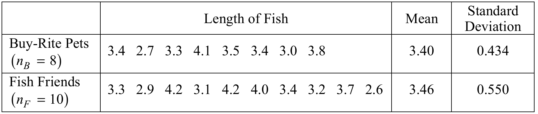
Let $\mu_{\text{B}}$ represent the population mean length of all adult fish of this species from Buy-Rite Pets, and let $\mu_{\text{F}}$ represent the population mean length of all adult fish of this species from Fish Friends.

The hypotheses to be tested are $\text{H}_0: \mu_{\text{B}} = \mu_{\text{F}}$ versus $\text{H}_{\text{a}}: \mu_{\text{B}} < \mu_{\text{F}}$.

Step 2: Identifies a correct test procedure (by name or by formula) and checks appropriate conditions

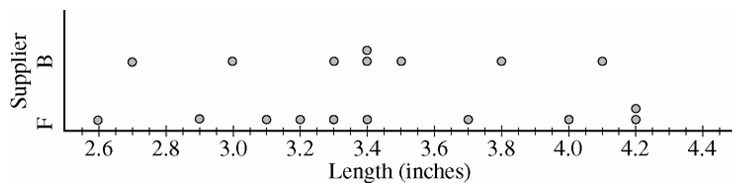
The appropriate test is a two-sample $t$-test. The first condition is that the samples are independent random samples from the two populations. This was stated in the question. The second condition is that the population distributions of fish lengths are normal. The following dotplots reveal no obvious departures from normality, so it appears reasonable to proceed with the two-sample $t$-test.

Step 3: Demonstrates correct mechanics, including the value of the test statistic, df and $p$-value (or rejection region)

The test statistic is: $t = \dfrac{\overline{x}_{\text{B}} – \overline{x}_{\text{F}}}{\sqrt{\dfrac{s_{\text{B}}^2}{n_{\text{B}}} + \dfrac{s_{\text{F}}^2}{n_{\text{F}}}}} = \dfrac{3.40 – 3.46}{\sqrt{\dfrac{0.434^2}{8} + \dfrac{0.550^2}{10}}} \approx -0.259$

With $\text{df} = 15.99999$, $p$-value $= 0.3996$.

Step 4: States a correct conclusion in the context of the problem, using the result of the statistical test

Because this $p$-value is larger than any conventional significance level (such as $\alpha = 0.10$ or $\alpha = 0.05$), we fail to reject $\text{H}_0$. The sample data do not provide convincing evidence to conclude that the mean length of the adult fish of the species from Fish Friends is greater than the mean length of the adult fish of the same species from Buy-Rite Pets.

Question

A manufacturer of toxic pesticide granules plans to use a dye to color the pesticide so that birds will avoid eating it. A series of experiments will be designed to find colors or patterns that three bird species (blackbirds, starlings, and geese) will avoid eating. Representative samples of birds will be captured to use in the experiments, and the response variable will be the amount of time a hungry bird will avoid eating food of a particular color or pattern.

(a) Previous research has shown that male birds do not avoid solid colors. However, it is possible that males might avoid colors displayed in a pattern, such as stripes. In an effort to prevent males from eating the pesticide, the following two treatments are applied to the pesticide granules.

Treatment 1: A red background with narrow blue stripes
Treatment 2: A blue background with narrow red stripes

To increase the power of detecting a difference in the two treatments in the analysis of the experiment, the researcher decided to block on the three species of birds (blackbirds, starlings, and geese). Assuming there are 100 birds of each of the three species, explain how you would assign birds to treatments in such a block design.

(b) Other than blocking, what could the researcher do to increase the power of detecting a difference in the two treatments in the analysis of the experiment? Explain how your approach would increase the power.

Most-appropriate topic codes (AP Statistics):

• Topic $1.13$ — Experimental Design (Part $\mathrm{a}$: randomized block design and random assignment)
• Topic $1.13$ — Experimental Design (Part $\mathrm{a}$: blocking on bird species to reduce variability)
• Topic $4.8$ — Justifying a Claim Based on a Confidence Interval for the Difference Between Two Population Means (Part $\mathrm{b}$: power and ability to detect treatment differences)
• Topic $4.10$ — Carrying Out a Test for the Difference Between Two Population Means (Part $\mathrm{b}$: factors affecting power, including sample size and significance level)

▶️ Answer/Explanation

(a)

Form three blocks based on species: Block 1 = blackbirds, Block 2 = starlings, Block 3 = geese. Since there are 100 birds of each species, each block contains 100 birds.
Within each block, randomly assign the 100 birds to the two treatments as follows:
Label each bird in the block with a unique number from 00 to 99. Use a random number table, calculator, or statistical software to generate a list of 50 distinct two-digit numbers between 00 and 99. The birds whose labels match these 50 numbers are assigned Treatment 1 (red background with narrow blue stripes). The remaining 50 birds in the block are assigned Treatment 2 (blue background with narrow red stripes).
Repeat this exact randomization procedure independently within Block 2 (starlings) and Block 3 (geese).
This results in 50 birds per treatment within each species block, and the random assignment ensures that any differences observed between treatments are not due to systematic differences among the birds.

(b)

One effective way to increase the power of the test (other than blocking) is to increase the sample size.
Increasing the number of birds in the study reduces the standard error of the sampling distribution of the difference in sample means.
A smaller standard error means the test statistic will be larger for any given true difference between treatments, making it more likely that the test will detect a real difference if one exists — that is, the power of the test increases.
Another valid approach is to increase the significance level $\alpha$ (for example, from $\alpha = 0.01$ to $\alpha = 0.05$). Raising $\alpha$ makes it easier to reject a false null hypothesis, which lowers the probability of a Type II error ($\beta$), and since power $= 1 – \beta$, the power increases.

Question

A serum cholesterol level above $250$ milligrams per deciliter (mg/dl) of blood is a risk factor for cardiovascular disease in humans. At a medical center in St. Louis, a study to test the effectiveness of a new cholesterol-lowering drug was conducted. One hundred people with cholesterol levels between $250$ mg/dl and $300$ mg/dl were available for this study. Fifty people were assigned at random to each of two treatment groups. One group received the standard cholesterol-lowering medication and the other group received the new drug. After taking the drug for three weeks, the $50$ subjects who received the standard treatment had a mean decrease in cholesterol level of $10$ mg/dl with a standard deviation of $8$ mg/dl, and the $50$ subjects who received the new drug had a mean decrease of $18$ mg/dl with a standard deviation of $12$ mg/dl.

Does the new drug appear to be more effective than the standard treatment in lowering mean cholesterol level? Give appropriate statistical evidence to support your conclusion.

Most-appropriate topic codes (AP Statistics):

• Topic 4.9 — Setting Up a Test for the Difference Between Two Population Means
• Topic 4.10 — Carrying Out a Test for the Difference Between Two Population Means

▶️ Answer/Explanation

Step 1: State the Hypotheses
Let $\mu_S$ = true mean decrease in cholesterol level for patients taking the standard drug
Let $\mu_N$ = true mean decrease in cholesterol level for patients taking the new drug
$H_0:\, \mu_S – \mu_N = 0$ (the two drugs are equally effective at lowering cholesterol
$H_a:\, \mu_S – \mu_N < 0$ (the new drug produces a greater mean decrease in cholesterol)

Step 2: Name the Test and Verify Conditions
Procedure: Two-sample $t$-test for the difference in population means.
• Random: Subjects were randomly assigned to the two treatment groups.
– Large Samples: Both sample sizes are large ($n_S = n_N = 50 \geq 30$), so by the Central Limit Theorem the sampling distribution of $\bar{x}_S – \bar{x}_N$ is approximately normal.
– Independence: The two treatment groups are independent of each other (separate random assignments, subjects cannot be in both groups).

Step 3: Calculate the Test Statistic

Given values: $\bar{x}_S = 10,\; s_S = 8,\; n_S = 50$ and $\bar{x}_N = 18,\; s_N = 12,\; n_N = 50$
$t = \dfrac{(\bar{x}_S – \bar{x}_N) – 0}{\sqrt{\dfrac{s_S^2}{n_S} + \dfrac{s_N^2}{n_N}}} = \dfrac{10 – 18}{\sqrt{\dfrac{8^2}{50} + \dfrac{12^2}{50}}}$
$= \dfrac{-8}{\sqrt{\dfrac{64}{50} + \dfrac{144}{50}}} = \dfrac{-8}{\sqrt{\dfrac{208}{50}}} = \dfrac{-8}{\sqrt{4.16}} \approx \dfrac{-8}{2.040} \approx -3.92$
Degrees of freedom (conservative): $df = \min(n_S – 1,\; n_N – 1) = \min(49,\; 49) = 49$
From the $t$-table at $df = 49$: since $|t| = 3.92$ exceeds the critical value $t^* = 3.496$ at tail probability $0.0005$,
$p\text{-value} < 0.001$

Step 4: State the Conclusion in Context
Since $p\text{-value} < 0.001 < \alpha = 0.05$, we reject $H_0$.
$\text{There is convincing statistical evidence that the new drug produces a greater mean decrease in cholesterol level than the standard treatment.}$
This question is a classic two-sample $t$-test, and the data make a strong case. The new drug group averaged a $18$ mg/dl drop in cholesterol versus only $10$ mg/dl for the standard treatment — an $8$ mg/dl difference that turns out to be far too large to chalk up to the luck of random assignment. With $t \approx -3.92$ and a $p$-value well below $0.001$, there’s less than a 1-in-1000 chance of seeing a gap this big if the drugs were truly equally effective. Crucially, because subjects were randomly assigned to treatment groups, we’re not just observing an association — we have solid grounds to conclude that the new drug is actually causing the greater cholesterol reduction.

Question

There have been many studies recently concerning coffee drinking and cholesterol level. While it is known that several coffee-bean components can elevate blood cholesterol level, it is thought that a new type of paper coffee filter may reduce the presence of some of these components in coffee.

The effect of the new filter on cholesterol level will be studied over a 10-week period using 300 nonsmokers who each drink 4 cups of caffeinated coffee per day. Each of these 300 participants will be assigned to one of two groups: the experimental group, who will only drink coffee that has been made with the new filter, or the control group, who will only drink coffee that has been made with the standard filter. Each participant’s cholesterol level will be measured at the beginning and at the end of the study.

(a) Describe an appropriate method for assigning the subjects to the two groups so that each group will have an equal number of subjects.

(b) In this study, the researchers chose to include a group who only drank coffee that was made with the standard filter. Why is it important to include a control group in this study even though cholesterol levels will be measured at the beginning and at the end of the study?

(c) Which test would you conduct to determine whether the change in cholesterol level would be greater if people used the new filter rather than using the standard filter?

(d) Why would the researchers choose to use only nonsmokers in the study?

Most-appropriate topic codes (AP Statistics):

• Topic 1.13 — Experimental Design (Parts a, b, d)
• Topic 4.10 — Carrying Out a Test for the Difference Between Two Population Means (Part c)
• Topic 4.9 — Setting Up a Test for the Difference Between Two Population Means (Part c)

▶️ Answer/Explanation

(a)

Assign each of the 300 subjects a unique number from 001 to 300.
Use a random number table or a random number generator to randomly select 150 of these numbers — the subjects corresponding to those numbers will be placed in the experimental group (new filter), and the remaining 150 subjects will be assigned to the control group (standard filter).
This ensures that each subject has an equal chance of being assigned to either group, and that both groups end up with exactly 150 subjects.

(b)

Without a control group, if cholesterol levels change over the 10-week period, there is no way to know whether the change was caused by the new filter or by some other factor that changed during that time — for example, seasonal changes in diet or physical activity.
Simply measuring cholesterol at the beginning and end for one group only tells us that a change occurred, but not why it occurred.
By including a control group using the standard filter, researchers can compare the mean change in cholesterol between the two groups, allowing them to attribute any difference specifically to the new filter rather than to an outside confounding variable.
In short, the control group is what makes it possible to isolate the effect of the new filter from other changes that might naturally occur over the 10-week period.

(c)

The appropriate test is the two-sample $t$-test for means (or equivalently, the two-sample $t$-test for mean differences).
This test compares the mean change in cholesterol level for the new-filter group against the mean change in cholesterol level for the standard-filter group, using two independent samples of size 150 each.

(d)

Smoking is known to be related to cholesterol level, so if the study included both smokers and nonsmokers, smoking status could act as an extraneous source of variability — making it harder to detect the true effect of the coffee filter.
By restricting the study to nonsmokers only, the researchers create more homogeneous groups, reducing variability within each group and allowing for a more precise and sensitive comparison of the filter’s effect on cholesterol.
This is similar in spirit to blocking — controlling for a known nuisance variable (smoking) so that it does not obscure the treatment effect, though it does mean the results can only be generalized to nonsmokers.

AP Statistics 4.10 Carrying Out a Test for the Difference Between Two Population Means- Exam Style Questions - FRQs - New Syllabus

Question

Question

Question

Question

Question

Question

Resources

Members

Company