AP Statistics 4.2 Constructing a Confidence Interval for a Population Mean or Population Mean Difference- Exam Style Questions - FRQs - New Syllabus

Question

A company sells a certain type of whistle. The price of the whistle varies from store to store. Julio, a statistician at the company, wants to estimate the mean price, in dollars ($\$\delta$), of this type of whistle at all stores that sell the whistle.

(a)
i. Identify the appropriate inference procedure for Julio to use.
ii. Describe the parameter for the inference procedure you identified in part (a-i) in context.

Julio called the managers of $20$ randomly selected stores that sell the whistle and recorded the price of the whistle at each store. Following is a dotplot of Julio’s data.

The summary statistics for Julio’s data are shown in the following table.

Summary Statistics for Julio’s Data

(b) Julio wants to examine some characteristics of the distribution of the sample of whistle prices.

i. Describe the shape of the distribution of the sample of whistle prices. Justify your response using appropriate values from the summary statistics table.
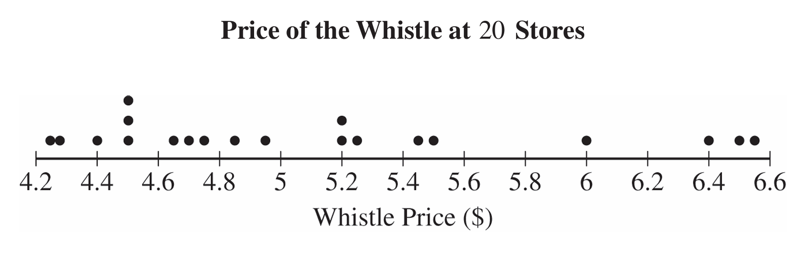
ii. Using the $1.5 \times \text{IQR}$ rule, determine whether there are any outliers in the sample of whistle prices. Justify your response.

It can often be difficult to determine whether the distribution of sample data is skewed by looking at a graph of the data and the summary statistics, particularly when the sample size is small. Thus, statisticians sometimes measure how skewed a data set is. One such measure is Pearson’s coefficient of skewness, which is calculated using the following formula.

$\text{Pearson’s Coefficient of Skewness} = \dfrac{3(\bar{x}-m)}{s}$

In the formula, $\bar{x}$ is the sample mean, $m$ is the sample median, and $s$ is the sample standard deviation.

(c)
i. Calculate Pearson’s coefficient of skewness for Julio’s sample of $20$ whistle prices. Show your work.

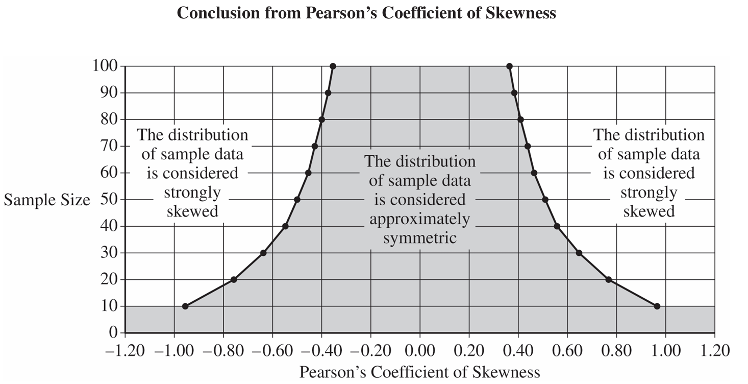The following graph shows conclusions that can be made about the shape of the distribution of sample data based on Pearson’s coefficient of skewness and sample size.

ii. Indicate the value of the Pearson’s coefficient of skewness you calculated in part (c-i) for the appropriate sample size by marking it with an “X” on the preceding graph.

(d) Consider your work in part (c).

i. What should you conclude about the shape of the distribution of the sample of whistle prices? Justify your response.

Julio’s inference procedure in part (a-i) needs one of the following requirements to be satisfied to verify the normality condition.
• The sample size is greater than or equal to $30$.
• If the sample size is less than $30$, the distribution of the sample data is not strongly skewed and does not have outliers.

ii. Using your response to (d-i) and the preceding requirements, is the normality condition satisfied for Julio’s data? Explain your response.

Most-appropriate topic codes (AP Statistics):

• Topic $1.7$ — Summary Statistics for One Quantitative Variable (Parts $ \mathrm{b} $, $ \mathrm{c} $)
• Topic $1.8$ — Graphical Representations of Summary Statistics for One Quantitative Variable (Parts $ \mathrm{b} $, $ \mathrm{c} $)
• Topic $4.2$ — Constructing a Confidence Interval for a Population Mean or Population Mean Difference (Parts $ \mathrm{a} $, $ \mathrm{d} $)

▶️ Answer/Explanation

(a)
i. Julio should use a one-sample $t$-interval for a population mean.
ii. The parameter of interest is $\mu$, the true mean price (in dollars) of this type of whistle at all stores that sell it.

(b)
i. The distribution of the sample of whistle prices is skewed to the right. This is because the mean ($5.12$) is greater than the median ($4.885$).
ii. $\text{IQR} = Q_3 – Q_1 = 5.475 – 4.51 = 0.965$.
Lower boundary: $Q_1 – 1.5(\text{IQR}) = 4.51 – 1.5(0.965) = 3.0625$.
Upper boundary: $Q_3 + 1.5(\text{IQR}) = 5.475 + 1.5(0.965) = 6.9225$.
Since the minimum value ($4.25$) is greater than $3.0625$ and the maximum value ($6.58$) is less than $6.9225$, there are no outliers in the sample.

(c)
i. $\text{Pearson’s Coefficient} = \dfrac{3(5.12 – 4.885)}{0.743} \approx 0.949$.
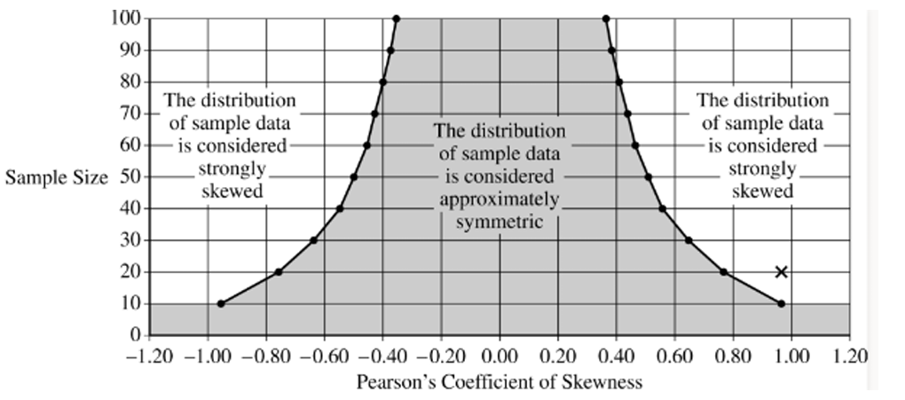
ii. On the graph, you would plot an “X” at a sample size of $y = 20$ and a skewness coefficient of $x \approx 0.949$.

(d)
i. We can conclude that the distribution of the sample of whistle prices is strongly skewed. This is justified because the calculated coefficient of $0.949$ for a sample size of $20$ falls in the “strongly skewed” region of the provided graph.
ii. No, the normality condition is not satisfied. The sample size ($n = 20$) is less than $30$, and although there are no outliers, the sample data is strongly skewed, failing the second condition.

Question

An environmental group conducted a study to determine whether crows in a certain region were ingesting food containing unhealthy levels of lead. A biologist classified lead levels greater than $6.0$ parts per million (ppm) as unhealthy. The lead levels of a random sample of $23$ crows in the region were measured and recorded. The data are shown in the stemplot below.

(a) What proportion of crows in the sample had lead levels that are classified by the biologist as unhealthy?

(b) The mean lead level of the $23$ crows in the sample was $4.90$ ppm and the standard deviation was $1.12$ ppm. Construct and interpret a $95$ percent confidence interval for the mean lead level of crows in the region.

Most-appropriate topic codes (AP Statistics):

• Topic $1.5$ — Graphical Representations for One Quantitative Variable (Part $ \mathrm{a} $)
• Topic $1.6$ — Descriptions for One Quantitative Variable Distributions (Part $ \mathrm{b} $ — checking normality condition)
• Topic $4.2$ — Constructing a Confidence Interval for a Population Mean or Population Mean Difference (Part $ \mathrm{b} $)
• Topic $4.3$ — Justifying a Claim Based on a Confidence Interval for a Population Mean or Population Mean Difference (Part $ \mathrm{b} $)

▶️ Answer/Explanation

(a)

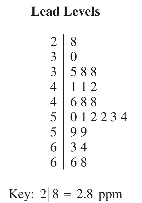
From the stemplot, the crows with lead levels greater than $6.0$ ppm are those with values $6.3,\ 6.4,\ 6.6,$ and $6.8$ ppm — that gives us exactly $4$ crows out of the $23$ sampled.
$\text{Proportion} = \frac{4}{23} \approx 0.174$
$\boxed{\dfrac{4}{23} \approx 0.174}$

(b)

Step 1: Identify the procedure and check conditions.
The appropriate procedure is a one-sample $t$-interval for a population mean, using the formula:
$\bar{x} \pm t^* \cdot \frac{s}{\sqrt{n}}$
Condition 1 — Random sample: The problem states the $23$ crows were randomly selected, so this condition is met.
Condition 2 — Normality: The sample size of $23$ is not large enough on its own, so we check the stemplot. The data show no strong skewness and no outliers, so it is reasonable to assume the population distribution of lead levels is approximately normal.

Step 2: Compute the confidence interval.
Given: $\bar{x} = 4.90$ ppm, $s = 1.12$ ppm, $n = 23$
Degrees of freedom: $df = n – 1 = 22$
Critical value at $95\%$ confidence with $22$ df: $t^* = 2.074$
$4.90 \pm 2.074 \times \frac{1.12}{\sqrt{23}}$
$4.90 \pm 2.074 \times 0.2336$
$4.90 \pm 0.484$
$\boxed{(4.416,\ 5.384) \text{ ppm}}$

Step 3: Interpret the interval.
We are $95\%$ confident that the true mean lead level among all crows in this region is between $4.416$ ppm and $5.384$ ppm.

Question

Independent random samples of 500 households were taken from a large metropolitan area in the United States for the years 1950 and 2000. Histograms of household size (number of people in a household) for the years are shown below.

(a) Compare the distributions of household size in the metropolitan area for the years 1950 and 2000.

(b) A researcher wants to use these data to construct a confidence interval to estimate the change in mean household size in the metropolitan area from the year 1950 to the year 2000. State the conditions for using a two-sample $t$-procedure, and explain whether the conditions for inference are met.

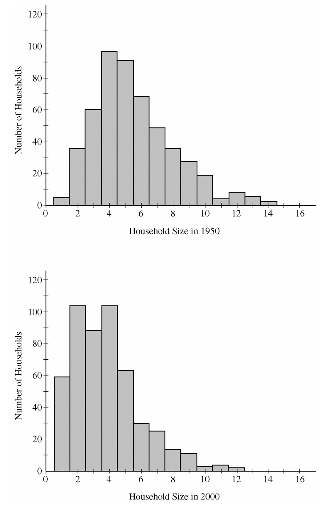
Most-appropriate topic codes (AP Statistics):

• Topic 1.9 — Comparisons of the Distributions for One Quantitative Variable (Part a)
• Topic 4.2 — Constructing a Confidence Interval for a Population Mean or Population Mean Difference (Part b)

▶️ Answer/Explanation

(a)
When comparing distributions, we address shape, center, spread, and any unusual features:
• Shape: Both distributions of household sizes are strongly skewed to the right (positively skewed).
• Center: The household sizes in 1950 typical center at a higher value than in 2000. The median household size in 1950 is approximately 4 people, whereas the median household size in 2000 has shifted downward to approximately 3 people.
• Spread: Household sizes were more variable in 1950 than in 2000. The total range for 1950 runs from 1 to 14 (a range of 13), while the range for 2000 is slightly narrower, running from 1 to 12 (a range of 11).
• Outliers/Features: Both time periods show a cluster of typical values between 1 and 6 people, but 1950 has a longer tail extending to very large households compared to 2000.

(b)
The conditions required for a two-sample $t$-procedure, along with verification, are outlined below:
1. Independent Random Sampling Condition: The data must come from two independent random samples.
• Status: Met. The problem states that “independent random samples of 500 households were taken.”
2. Normality Condition: The populations should be normally distributed, or the sample sizes must be large enough to apply the Central Limit Theorem.
• Status: Met. Even though both histograms show distinct right-skewness, the sample sizes are $n_{1950} = 500$ and $n_{2000} = 500$. Since both sample sizes are well above the threshold of 30 ($500 \ge 30$), the Central Limit Theorem ensures that the sampling distribution of the difference in sample means is approximately normal.
3. Independence (10% Rule) Condition: The sample sizes should not exceed 10% of their respective population sizes if sampling without replacement.
• Status: Met. It is highly reasonable to assume that 500 households is less than 10% of all available households in a “large metropolitan area” in the United States for both 1950 and 2000.

Question

A car manufacturer is interested in conducting a study to estimate the mean stopping distance for a new type of brakes when used in a car that is traveling at 60 miles per hour. These new brakes will be installed on cars of the same model and the stopping distance will be observed. The cost of each observation is $\$100$. A budget of $\$12{,}000$ is available to conduct the study and the goal is to carry it out in the most economical way possible. Preliminary studies indicate that $\sigma = 12$ feet for stopping distances.

(a) Are sufficient funds available to estimate the mean stopping distance to within $2$ feet of the true mean stopping distance with $95\%$ confidence?

Explain your answer.

(b) A regulatory agency requires a $95\%$ level of confidence for an estimate of mean stopping distance that is within $2$ feet of the true mean stopping distance. The car manufacturer cannot exceed the budget of $\$12{,}000$ for the study. Discuss the consequences of these constraints.

Most-appropriate topic codes (AP Statistics):

• Topic 4.2 — Constructing a Confidence Interval for a Population Mean or Population Mean Difference (Parts $\mathrm{a}$, $\mathrm{b}$)
• Topic 4.1 — Sampling Distributions for Sample Means (Part $\mathrm{a}$)

▶️ Answer/Explanation

(a)
No, sufficient funds are not available.
To estimate the mean to within a margin of error $E = 2$ feet with $95\%$ confidence, we use the sample size formula:
$n = \left(\frac{z^* \cdot \sigma}{E}\right)^2$
With $z^* = 1.96$, $\sigma = 12$, and $E = 2$:
$n = \left(\frac{1.96 \times 12}{2}\right)^2 = \left(\frac{23.52}{2}\right)^2 = (11.76)^2 = 138.3$
Since sample size must be a whole number, we round up:
$\boxed{n = 139}$
The cost of conducting 139 observations would be:
$139 \times \$100 = \$13{,}900$
Since $\$13{,}900 > \$12{,}000$, the budget is insufficient to achieve the desired margin of error.
Alternatively, with a budget of $\$12{,}000$, the manufacturer can afford at most:
$n = \frac{\$12{,}000}{\$100} = 120 \text{ observations}$
The margin of error achievable with $n = 120$ is:
$E = 1.96 \times \frac{12}{\sqrt{120}} = 1.96 \times 1.095 \approx 2.15 \text{ feet}$
Since $2.15 > 2$, the required precision of $2$ feet cannot be met with the available budget.
$\boxed{\text{Sufficient funds are NOT available}}$

(b)
The two constraints — a $95\%$ confidence level with a margin of error within $2$ feet, and a budget cap of $\$12{,}000$ — are in direct conflict with each other.
Meeting the regulatory agency’s requirement demands at least $139$ observations, which costs $\$13{,}900$. The budget of $\$12{,}000$ only allows $120$ observations, which yields a margin of error of approximately $2.15$ feet at the $95\%$ confidence level.
Since $2.15 > 2$, the manufacturer cannot simultaneously satisfy both the statistical requirement (within $2$ feet) and the financial constraint ($\$12{,}000$ budget).
As a consequence, the car manufacturer will not be able to meet the regulatory agency’s requirements with the allocated budget. Unless the budget is increased to at least $\$13{,}900$, or the agency relaxes its precision requirement, the manufacturer cannot obtain regulatory approval under the current constraints.
$\boxed{\text{The manufacturer cannot meet the regulatory requirement within the given budget}}$

Question

A researcher believes that treating seeds with certain additives before planting can enhance the growth of plants. An experiment to investigate this is conducted in a greenhouse. From a large number of Roma tomato seeds, 24 seeds are randomly chosen and 2 are assigned to each of 12 containers. One of the 2 seeds is randomly selected and treated with the additive. The other seed serves as a control. Both seeds are then planted in the same container. The growth, in centimeters, of each of the 24 plants is measured after 30 days. These data were used to generate the partial computer output shown below. Graphical displays indicate that the assumption of normality is not unreasonable.

(a) Construct a confidence interval for the mean difference in growth, in centimeters, of the plants from the untreated and treated seeds. Be sure to interpret this interval.

(b) Based only on the confidence interval in part (a), is there sufficient evidence to conclude that there is a significant mean difference in growth of the plants from untreated seeds and the plants from treated seeds? Justify your conclusion.

Most-appropriate topic codes (AP Statistics):

• Topic 4.2 — Constructing a Confidence Interval for a Population Mean or Population Mean Difference (Part a)
• Topic 4.3 — Justifying a Claim Based on a Confidence Interval for a Population Mean or Population Mean Difference (Part b)
• Topic 1.13 — Experimental Design (Matched-pairs design context)

▶️ Answer/Explanation

(a)

Step 1 — Identify the appropriate procedure:
Since the data consist of paired observations (one treated and one untreated seed per container), we use a one-sample $t$-confidence interval for the mean of the differences:
$ \bar{d} \pm t^* \cdot \frac{s_d}{\sqrt{n}} $
Step 2 — Check conditions:
The 24 seeds were randomly chosen and randomly assigned within each container, so the differences are independent. The problem states that graphical displays indicate normality is not unreasonable, so the condition for using a $t$-procedure is satisfied.
Step 3 — Compute the interval:
From the computer output: $\bar{d} = -2.015$, $s_d = 1.163$, $n = 12$.
Degrees of freedom: $df = n – 1 = 11$.
For a 95% confidence interval, the critical value is $t^* = 2.201$ (from the $t$-table with $df = 11$).
$ \bar{d} \pm t^* \cdot \frac{s_d}{\sqrt{n}} = -2.015 \pm 2.201 \times \frac{1.163}{\sqrt{12}} $
$ = -2.015 \pm 2.201 \times 0.336 $
$ = -2.015 \pm 0.739 $
$ \boxed{(-2.754,\ -1.276)} $

Step 4 — Interpret the interval:
We are 95% confident that the true mean difference in growth (untreated minus treated) is between $-2.754$ cm and $-1.276$ cm. In other words, on average, the untreated plants grew between about 1.28 cm and 2.75 cm less than the treated plants.

(b)

Step 1 — State the hypotheses (for reference):
$ H_0: \mu_d = 0 \quad \text{vs.} \quad H_a: \mu_d \neq 0 $
where $\mu_d$ is the true mean difference in growth between untreated and treated seeds.

Step 2 — Draw the conclusion:
Yes, there is sufficient evidence of a significant mean difference in growth. The 95% confidence interval $(-2.754,\ -1.276)$ does not contain zero. Since zero — the value that would indicate no difference — falls entirely outside the interval, we can reject $H_0$ at the $\alpha = 0.05$ significance level. The data provide convincing statistical evidence that the additive treatment produces greater growth than the control, with treated plants growing meaningfully taller on average.

Question

A pharmaceutical company has developed a new drug to reduce cholesterol. A regulatory agency will recommend the new drug for use if there is convincing evidence that the mean reduction in cholesterol level after one month of use is more than 20 milligrams/deciliter (mg/dl), because a mean reduction of this magnitude would be greater than the mean reduction for the current most widely used drug.

The pharmaceutical company collected data by giving the new drug to a random sample of 50 people from the population of people with high cholesterol. The reduction in cholesterol level after one month of use was recorded for each individual in the sample, resulting in a sample mean reduction and standard deviation of 24 mg/dl and 15 mg/dl, respectively.

(a) The regulatory agency decides to use an interval estimate for the population mean reduction in cholesterol level for the new drug. Provide this 95 percent confidence interval. Be sure to interpret this interval.

(b) Because the 95 percent confidence interval includes 20, the regulatory agency is not convinced that the new drug is better than the current best-seller. The pharmaceutical company tested the following hypotheses.

$H_0: \mu = 20$ versus $H_a: \mu > 20$,

where $\mu$ represents the population mean reduction in cholesterol level for the new drug.

The test procedure resulted in a $t$-value of 1.89 and a $p$-value of 0.033. Because the $p$-value was less than 0.05, the company believes that there is convincing evidence that the mean reduction in cholesterol level for the new drug is more than 20. Explain why the confidence interval and the hypothesis test led to different conclusions.

(c) The company would like to determine a value $L$ that would allow them to make the following statement.

We are 95 percent confident that the true mean reduction in cholesterol level is greater than $L$.

A statement of this form is called a one-sided confidence interval. The value of $L$ can be found using the following formula.

\[L = \bar{x} – t^* \dfrac{s}{\sqrt{n}}\]

This has the same form as the lower endpoint of the confidence interval in part (a), but requires a different critical value, $t^*$. What value should be used for $t^*$?

Recall that the sample mean reduction in cholesterol level and standard deviation are 24 mg/dl and 15 mg/dl, respectively. Compute the value of $L$.

(d) If the regulatory agency had used the one-sided confidence interval in part (c) rather than the interval constructed in part (a), would it have reached a different conclusion? Explain.

Most-appropriate topic codes (AP Statistics):

• Topic 4.2 — Constructing a Confidence Interval for a Population Mean or Population Mean Difference (Part a)
• Topic 4.4 — Setting Up a Test for a Population Mean or Population Mean Difference (Part b)
• Topic 4.5 — Carrying Out a Test for a Population Mean or Population Mean Difference (Part b)
• Topic 4.2 — Constructing a Confidence Interval for a Population Mean or Population Mean Difference (Part c)
• Topic 4.3 — Justifying a Claim Based on a Confidence Interval for a Population Mean or Population Mean Difference (Parts c, d)

▶️ Answer/Explanation

(a)
The appropriate procedure is a one-sample $t$-interval for the population mean $\mu$.
Conditions:
— The data come from a random sample of 50 people.
— $\sigma$ is unknown; using the sample standard deviation $s = 15$.
— $n = 50 \geq 30$, so by the Central Limit Theorem the sampling distribution of $\bar{x}$ is approximately normal.
Given: $\bar{x} = 24$, $s = 15$, $n = 50$, and $df = 49$. For a 95% confidence interval, $t^* \approx 2.009$ (using $df = 49$).
The confidence interval formula is:
$\bar{x} \pm t^* \cdot \dfrac{s}{\sqrt{n}}$
$24 \pm 2.009 \cdot \dfrac{15}{\sqrt{50}}$
$24 \pm 2.009 \times 2.121$
$24 \pm 4.262$
$\boxed{(19.738,\ 28.262) \text{ mg/dl}}$
Interpretation: We are 95% confident that the true population mean reduction in cholesterol level after one month of use of the new drug is between approximately 19.7 mg/dl and 28.3 mg/dl.

(b)
The confidence interval and the hypothesis test led to different conclusions because they are based on different types of procedures that correspond to different questions being asked.
The 95% two-sided confidence interval is equivalent to a two-sided hypothesis test at $\alpha = 0.05$. The two-sided $p$-value for testing $H_0: \mu = 20$ against $H_a: \mu \neq 20$ would be $2 \times 0.033 = 0.066$, which exceeds $\alpha = 0.05$ — hence the confidence interval (which captures values consistent with a two-sided test) includes 20 and fails to reject $H_0$ at the 0.05 level.
The hypothesis test, however, is one-sided ($H_a: \mu > 20$) with a one-sided $p$-value of $0.033 < 0.05$, which leads to rejecting $H_0$. A one-sided test is more powerful in the direction specified and uses only one tail of the distribution. The two procedures are therefore testing different things, and it is the mismatch — using a two-sided interval to evaluate a one-sided hypothesis — that creates the apparent contradiction in conclusions.
$\boxed{\text{Two-sided CI} \leftrightarrow \text{two-sided test (}p = 0.066 > 0.05\text{)}; \quad \text{one-sided test: }p = 0.033 < 0.05}$

(c)
For a one-sided 95% confidence interval, we need to find $t^*$ such that 95% of the $t$-distribution with $df = 49$ lies above $-t^*$ (i.e., only one tail of area 0.05).
This corresponds to a tail probability of $p = 0.05$ (one tail) with $df = 49$. From the $t$-table:
$\boxed{t^* = 1.676 \quad (df = 49,\ \text{one tail}, \ \alpha = 0.05)}$
Now compute $L$:
$L = \bar{x} – t^* \cdot \dfrac{s}{\sqrt{n}} = 24 – 1.676 \cdot \dfrac{15}{\sqrt{50}}$
$= 24 – 1.676 \times 2.121$
$= 24 – 3.555$
$\boxed{L \approx 20.4 \text{ mg/dl}}$
Interpretation: We are 95% confident that the true mean reduction in cholesterol level after one month of use of the new drug is greater than approximately 20.4 mg/dl.

(d)
Yes, the regulatory agency would have reached a different conclusion using the one-sided confidence interval. The one-sided interval shows that the agency can be 95% confident that the true mean reduction is greater than $L \approx 20.4$ mg/dl, which is already above the threshold of 20 mg/dl required for recommendation. Since the entire range of plausible values for $\mu$ under the one-sided interval lies above 20, the agency would have had convincing evidence that the new drug reduces cholesterol by more than 20 mg/dl on average — and would therefore have recommended the drug for use.
$\boxed{L \approx 20.4 > 20 \Rightarrow \text{Yes, different conclusion: agency would recommend the drug}}$

Question

A researcher thinks that modern Thai dogs may be descendants of golden jackals. A random sample of 16 animals was collected from each of the two populations. The length (in millimeters) of the mandible (jawbone) was measured for each animal. The lower quartile, median, and upper quartile for each sample are shown in the table below, along with all values below the lower quartile and all values above the upper quartile.

(a) Display parallel boxplots of mandible lengths (showing outliers, if any) for the modern Thai dogs and the golden jackals on the grid below.

Based on the boxplots, write a few sentences comparing the distributions of mandible lengths for the two types of dogs.

(b) Is it reasonable to use the sample of mandible lengths of modern Thai dogs to construct an interval estimate of the mean mandible length for the population of modern Thai dogs? Justify your answer. (Note: You do not have to compute the interval.)

(c) Is it reasonable to use the sample data of mandible lengths of modern Thai dogs and the sample data of mandible lengths of golden jackals to perform a two-sample $t$-test for the difference in mean mandible lengths for the two types of dogs? Justify your answer. (Note: You do not have to conduct the test.)

Most-appropriate topic codes (AP Statistics):

• Topic 1.8 — Graphical Representations of Summary Statistics for One Quantitative Variable (Part a)
• Topic 1.9 — Comparisons of the Distributions for One Quantitative Variable (Part a)
• Topic 4.2 — Constructing a Confidence Interval for a Population Mean or Population Mean Difference (Part b)
• Topic 4.4 — Setting Up a Test for a Population Mean or Population Mean Difference (Part c)

▶️ Answer/Explanation

(a)

First, we check for outliers in each sample using the $1.5 \times \text{IQR}$ rule.
Modern Thai Dogs:
$\text{IQR} = Q_3 – Q_1 = 128 – 121 = 7$
Lower fence: $121 – 1.5(7) = 121 – 10.5 = 110.5$
Upper fence: $128 + 1.5(7) = 128 + 10.5 = 138.5$
All values (minimum = 114, maximum = 132) fall within these fences. No outliers.
Golden Jackals:
$\text{IQR} = Q_3 – Q_1 = 112 – 107 = 5$
Lower fence: $107 – 1.5(5) = 107 – 7.5 = 99.5$
Upper fence: $112 + 1.5(5) = 112 + 7.5 = 119.5$
Values 122, 124, and 125 exceed the upper fence of 119.5. Outliers: 122, 124, 125.
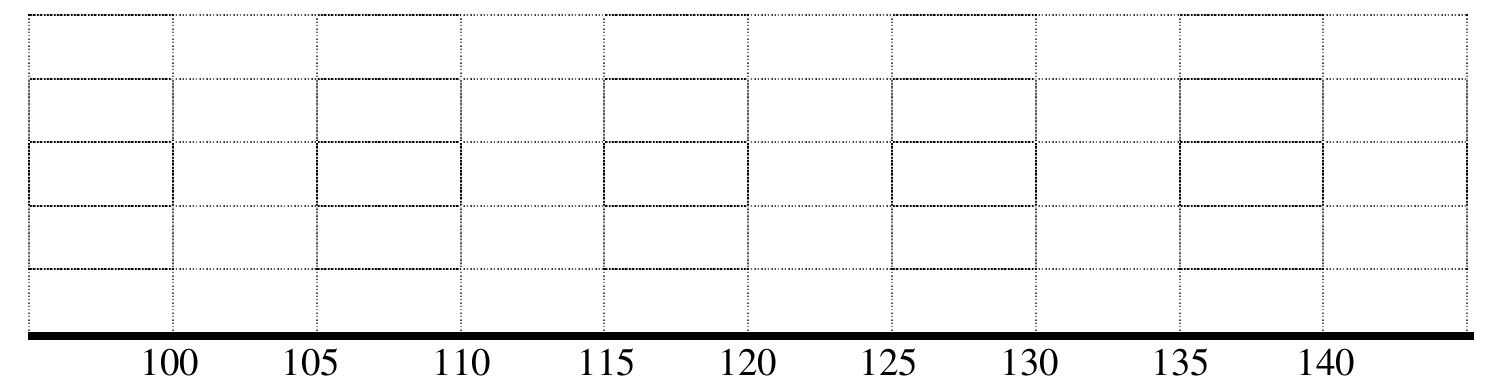
The parallel boxplots (with the scale from 100 to 140 mm) are shown below:

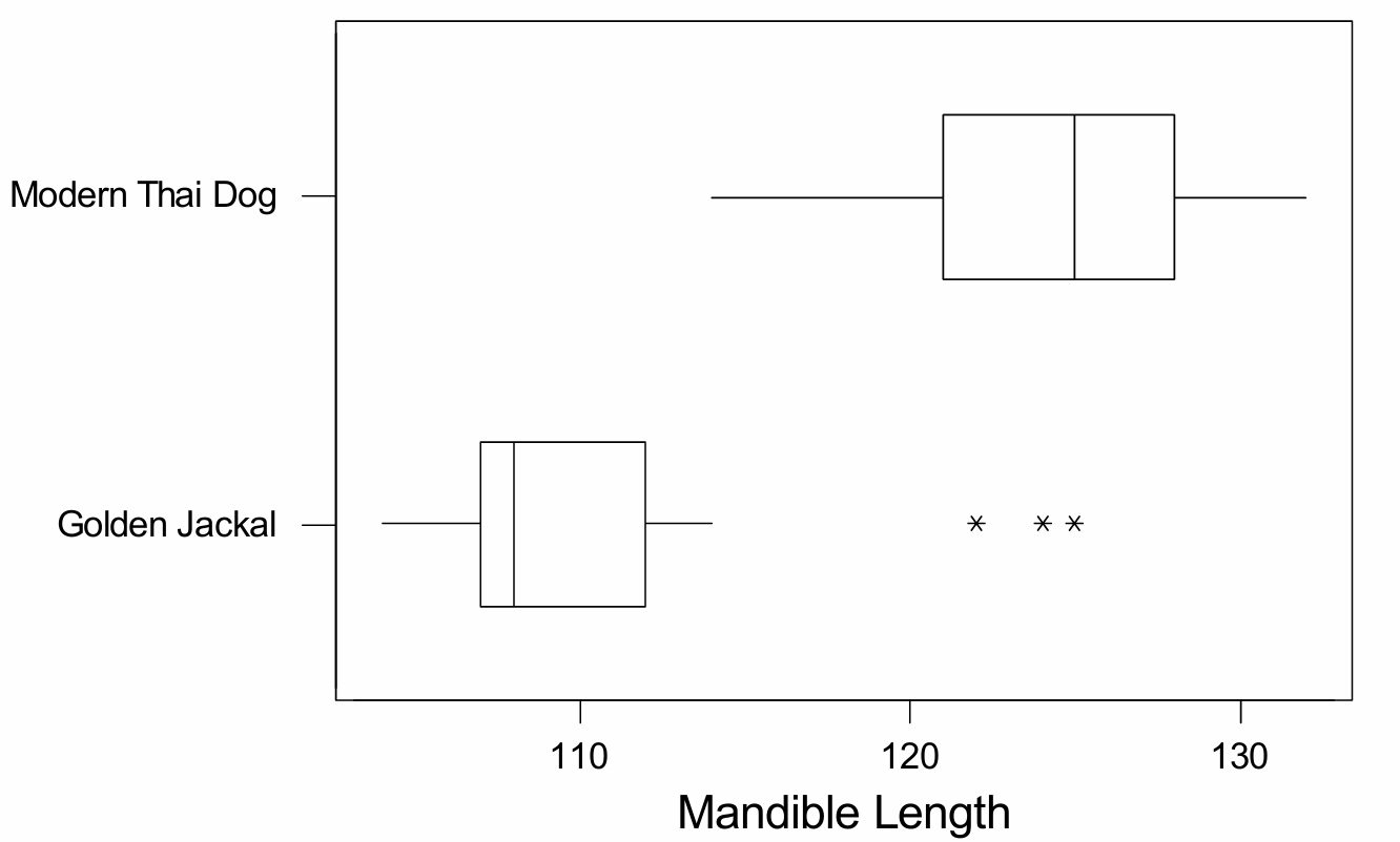
Comparison of distributions: The distributions of mandible lengths for modern Thai dogs and golden jackals are quite different. Modern Thai dogs have a much larger typical mandible length — a median of 125 mm — compared to golden jackals, whose median is only 108 mm. The distribution for modern Thai dogs appears approximately symmetric with no outliers, whereas the distribution for golden jackals is heavily skewed to the right, with three high outliers (122, 124, and 125 mm). The variability (spread) of the two distributions is roughly similar in terms of IQR, but the overall range for golden jackals is larger once the outliers are included.

(b)

Yes, it is reasonable to construct a $t$-confidence interval for the mean mandible length of modern Thai dogs. The boxplot for this sample is roughly symmetric with no outliers, which provides support for the assumption that the underlying population distribution is approximately normal. Since the data come from a random sample and the normality condition is reasonably satisfied even with a sample size of only 16, using a one-sample $t$-interval is appropriate here.

(c)

No, it would not be reasonable to perform a two-sample $t$-test using both groups. While the modern Thai dog sample looks approximately normal, the golden jackal sample is clearly not. The boxplot for golden jackals is strongly skewed to the right and contains three high outliers (122, 124, 125) in a sample of only 16 animals — a substantial proportion of the data. With such a small sample size, the $t$-test is not robust enough to overcome this serious departure from normality, so the normality condition required for the two-sample $t$-test is not reasonably met for the golden jackal population. Therefore, performing the two-sample $t$-test with this data would not be appropriate.

AP Statistics 4.2 Constructing a Confidence Interval for a Population Mean or Population Mean Difference- Exam Style Questions - FRQs - New Syllabus

Question

Question

Question

Question

Question

Question

Question

Resources

Members

Company