AP Statistics 4.3 Justifying a Claim Based on a Confidence Interval for a Population Mean or Population Mean Difference- Exam Style Questions - FRQs - New Syllabus

Question

According to a 2017 national survey in Country B, the mean number of bedrooms in newly built houses was 2.9. Rodney, a researcher, believes the mean number of bedrooms in newly built houses in the country was different in 2024 than it was in 2017. To investigate his belief, he took a large random sample of newly built houses in Country B in 2024 and recorded the number of bedrooms in each house. The distribution of the number of bedrooms for the sampled houses is summarized in the table.

Distribution of the Number of Bedrooms for the Houses Sampled in 2024

i. A house from the sample will be selected at random. What is the probability that the house had fewer than 3 bedrooms? Show your work.
ii. What is the mean number of bedrooms for the sample of newly built houses in 2024? Show your work.

B. Rodney will use a one-sample t-test for a population mean to test his belief.

i. In the context of Rodney’s investigation, state the hypotheses for the test.
ii. Explain, in context, what a Type I error would be for Rodney’s hypothesis test.

C. A different researcher, Keisha, suggests using a confidence interval to investigate whether the mean number of bedrooms in newly built houses in 2024 in Country B was different from 2.9. Assume the conditions for inference have been met. Using Rodney’s data, Keisha calculated a one-sample 97 percent confidence interval to estimate the population mean as $(3.01, 3.19)$. Based on the confidence interval, what conclusion can be made for Rodney’s hypothesis test in part B at $\alpha = 0.03$? Justify your answer.

Most-appropriate topic codes (AP Statistics):

• Topic $1.7$ — Summary Statistics for One Quantitative Variable (Part $ \mathrm{A} $)
• Topic $2.9$ — Parameters of Random Variables (Part $ \mathrm{A} $)
• Topic $4.3$ — Justifying a Claim Based on a Confidence Interval for a Population Mean or Population Mean Difference (Parts $ \mathrm{B} $, $ \mathrm{C} $)
• Topic $4.4$ — Setting Up a Test for a Population Mean or Population Mean Difference (Part $ \mathrm{B} $)

▶️ Answer/Explanation

A. i.
Fewer than 3 bedrooms means a house has either 1 or 2 bedrooms.
$P(\text{Bedrooms} < 3) = P(1) + P(2) = 0.12 + 0.22$
$\boxed{P(\text{Bedrooms} < 3) = 0.34}$

A. ii.
The sample mean is calculated by summing the products of the values and their corresponding proportions.
$\bar{x} = \sum x_i \cdot p_i = 1(0.12) + 2(0.22) + 3(0.28) + 4(0.22) + 5(0.14) + 6(0.02)$
$\bar{x} = 0.12 + 0.44 + 0.84 + 0.88 + 0.70 + 0.12$
$\boxed{\bar{x} = 3.10\,\text{bedrooms}}$

B. i.
Let $\mu$ represent the true mean number of bedrooms in all newly built houses in Country B in 2024.
$H_0: \mu = 2.9$
$H_a: \mu \neq 2.9$

B. ii.
• A Type I error happens if Rodney concludes that the true mean number of bedrooms in 2024 is different from 2.9 when, in reality, it is still exactly 2.9.
• In practice, this means the researcher would mistakenly declare a shift in housing layout profiles where no genuine structural trend modification occurred.

C.
• Since the significance level $\alpha = 0.03$ matches the two-sided boundary of a 97% confidence interval $(1 – 0.97 = 0.03)$, we can judge the test based on whether the null value falls inside the interval boundaries.
• The hypothesized baseline mean value $\mu_0 = 2.9$ lies completely outside Keisha’s 97% confidence interval of $(3.01, 3.19)$.
• Therefore, Rodney would reject the null hypothesis $H_0$ and conclude that there is convincing statistical evidence that the true mean number of bedrooms in newly built houses in Country B in 2024 is different from 2.9.

Question

An environmental group conducted a study to determine whether crows in a certain region were ingesting food containing unhealthy levels of lead. A biologist classified lead levels greater than $6.0$ parts per million (ppm) as unhealthy. The lead levels of a random sample of $23$ crows in the region were measured and recorded. The data are shown in the stemplot below.

(a) What proportion of crows in the sample had lead levels that are classified by the biologist as unhealthy?

(b) The mean lead level of the $23$ crows in the sample was $4.90$ ppm and the standard deviation was $1.12$ ppm. Construct and interpret a $95$ percent confidence interval for the mean lead level of crows in the region.

Most-appropriate topic codes (AP Statistics):

• Topic $1.5$ — Graphical Representations for One Quantitative Variable (Part $ \mathrm{a} $)
• Topic $1.6$ — Descriptions for One Quantitative Variable Distributions (Part $ \mathrm{b} $ — checking normality condition)
• Topic $4.2$ — Constructing a Confidence Interval for a Population Mean or Population Mean Difference (Part $ \mathrm{b} $)
• Topic $4.3$ — Justifying a Claim Based on a Confidence Interval for a Population Mean or Population Mean Difference (Part $ \mathrm{b} $)

▶️ Answer/Explanation

(a)

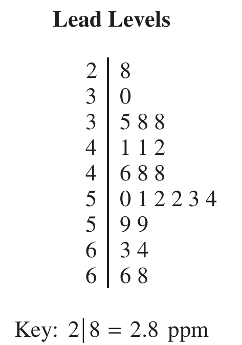
From the stemplot, the crows with lead levels greater than $6.0$ ppm are those with values $6.3,\ 6.4,\ 6.6,$ and $6.8$ ppm — that gives us exactly $4$ crows out of the $23$ sampled.
$\text{Proportion} = \frac{4}{23} \approx 0.174$
$\boxed{\dfrac{4}{23} \approx 0.174}$

(b)

Step 1: Identify the procedure and check conditions.
The appropriate procedure is a one-sample $t$-interval for a population mean, using the formula:
$\bar{x} \pm t^* \cdot \frac{s}{\sqrt{n}}$
Condition 1 — Random sample: The problem states the $23$ crows were randomly selected, so this condition is met.
Condition 2 — Normality: The sample size of $23$ is not large enough on its own, so we check the stemplot. The data show no strong skewness and no outliers, so it is reasonable to assume the population distribution of lead levels is approximately normal.

Step 2: Compute the confidence interval.
Given: $\bar{x} = 4.90$ ppm, $s = 1.12$ ppm, $n = 23$
Degrees of freedom: $df = n – 1 = 22$
Critical value at $95\%$ confidence with $22$ df: $t^* = 2.074$
$4.90 \pm 2.074 \times \frac{1.12}{\sqrt{23}}$
$4.90 \pm 2.074 \times 0.2336$
$4.90 \pm 0.484$
$\boxed{(4.416,\ 5.384) \text{ ppm}}$

Step 3: Interpret the interval.
We are $95\%$ confident that the true mean lead level among all crows in this region is between $4.416$ ppm and $5.384$ ppm.

Question

A researcher believes that treating seeds with certain additives before planting can enhance the growth of plants. An experiment to investigate this is conducted in a greenhouse. From a large number of Roma tomato seeds, 24 seeds are randomly chosen and 2 are assigned to each of 12 containers. One of the 2 seeds is randomly selected and treated with the additive. The other seed serves as a control. Both seeds are then planted in the same container. The growth, in centimeters, of each of the 24 plants is measured after 30 days. These data were used to generate the partial computer output shown below. Graphical displays indicate that the assumption of normality is not unreasonable.

(a) Construct a confidence interval for the mean difference in growth, in centimeters, of the plants from the untreated and treated seeds. Be sure to interpret this interval.

(b) Based only on the confidence interval in part (a), is there sufficient evidence to conclude that there is a significant mean difference in growth of the plants from untreated seeds and the plants from treated seeds? Justify your conclusion.

Most-appropriate topic codes (AP Statistics):

• Topic 4.2 — Constructing a Confidence Interval for a Population Mean or Population Mean Difference (Part a)
• Topic 4.3 — Justifying a Claim Based on a Confidence Interval for a Population Mean or Population Mean Difference (Part b)
• Topic 1.13 — Experimental Design (Matched-pairs design context)

▶️ Answer/Explanation

(a)

Step 1 — Identify the appropriate procedure:
Since the data consist of paired observations (one treated and one untreated seed per container), we use a one-sample $t$-confidence interval for the mean of the differences:
$ \bar{d} \pm t^* \cdot \frac{s_d}{\sqrt{n}} $
Step 2 — Check conditions:
The 24 seeds were randomly chosen and randomly assigned within each container, so the differences are independent. The problem states that graphical displays indicate normality is not unreasonable, so the condition for using a $t$-procedure is satisfied.
Step 3 — Compute the interval:
From the computer output: $\bar{d} = -2.015$, $s_d = 1.163$, $n = 12$.
Degrees of freedom: $df = n – 1 = 11$.
For a 95% confidence interval, the critical value is $t^* = 2.201$ (from the $t$-table with $df = 11$).
$ \bar{d} \pm t^* \cdot \frac{s_d}{\sqrt{n}} = -2.015 \pm 2.201 \times \frac{1.163}{\sqrt{12}} $
$ = -2.015 \pm 2.201 \times 0.336 $
$ = -2.015 \pm 0.739 $
$ \boxed{(-2.754,\ -1.276)} $

Step 4 — Interpret the interval:
We are 95% confident that the true mean difference in growth (untreated minus treated) is between $-2.754$ cm and $-1.276$ cm. In other words, on average, the untreated plants grew between about 1.28 cm and 2.75 cm less than the treated plants.

(b)

Step 1 — State the hypotheses (for reference):
$ H_0: \mu_d = 0 \quad \text{vs.} \quad H_a: \mu_d \neq 0 $
where $\mu_d$ is the true mean difference in growth between untreated and treated seeds.

Step 2 — Draw the conclusion:
Yes, there is sufficient evidence of a significant mean difference in growth. The 95% confidence interval $(-2.754,\ -1.276)$ does not contain zero. Since zero — the value that would indicate no difference — falls entirely outside the interval, we can reject $H_0$ at the $\alpha = 0.05$ significance level. The data provide convincing statistical evidence that the additive treatment produces greater growth than the control, with treated plants growing meaningfully taller on average.

Question

A pharmaceutical company has developed a new drug to reduce cholesterol. A regulatory agency will recommend the new drug for use if there is convincing evidence that the mean reduction in cholesterol level after one month of use is more than 20 milligrams/deciliter (mg/dl), because a mean reduction of this magnitude would be greater than the mean reduction for the current most widely used drug.

The pharmaceutical company collected data by giving the new drug to a random sample of 50 people from the population of people with high cholesterol. The reduction in cholesterol level after one month of use was recorded for each individual in the sample, resulting in a sample mean reduction and standard deviation of 24 mg/dl and 15 mg/dl, respectively.

(a) The regulatory agency decides to use an interval estimate for the population mean reduction in cholesterol level for the new drug. Provide this 95 percent confidence interval. Be sure to interpret this interval.

(b) Because the 95 percent confidence interval includes 20, the regulatory agency is not convinced that the new drug is better than the current best-seller. The pharmaceutical company tested the following hypotheses.

$H_0: \mu = 20$ versus $H_a: \mu > 20$,

where $\mu$ represents the population mean reduction in cholesterol level for the new drug.

The test procedure resulted in a $t$-value of 1.89 and a $p$-value of 0.033. Because the $p$-value was less than 0.05, the company believes that there is convincing evidence that the mean reduction in cholesterol level for the new drug is more than 20. Explain why the confidence interval and the hypothesis test led to different conclusions.

(c) The company would like to determine a value $L$ that would allow them to make the following statement.

We are 95 percent confident that the true mean reduction in cholesterol level is greater than $L$.

A statement of this form is called a one-sided confidence interval. The value of $L$ can be found using the following formula.

\[L = \bar{x} – t^* \dfrac{s}{\sqrt{n}}\]

This has the same form as the lower endpoint of the confidence interval in part (a), but requires a different critical value, $t^*$. What value should be used for $t^*$?

Recall that the sample mean reduction in cholesterol level and standard deviation are 24 mg/dl and 15 mg/dl, respectively. Compute the value of $L$.

(d) If the regulatory agency had used the one-sided confidence interval in part (c) rather than the interval constructed in part (a), would it have reached a different conclusion? Explain.

Most-appropriate topic codes (AP Statistics):

• Topic 4.2 — Constructing a Confidence Interval for a Population Mean or Population Mean Difference (Part a)
• Topic 4.4 — Setting Up a Test for a Population Mean or Population Mean Difference (Part b)
• Topic 4.5 — Carrying Out a Test for a Population Mean or Population Mean Difference (Part b)
• Topic 4.2 — Constructing a Confidence Interval for a Population Mean or Population Mean Difference (Part c)
• Topic 4.3 — Justifying a Claim Based on a Confidence Interval for a Population Mean or Population Mean Difference (Parts c, d)

▶️ Answer/Explanation

(a)
The appropriate procedure is a one-sample $t$-interval for the population mean $\mu$.
Conditions:
— The data come from a random sample of 50 people.
— $\sigma$ is unknown; using the sample standard deviation $s = 15$.
— $n = 50 \geq 30$, so by the Central Limit Theorem the sampling distribution of $\bar{x}$ is approximately normal.
Given: $\bar{x} = 24$, $s = 15$, $n = 50$, and $df = 49$. For a 95% confidence interval, $t^* \approx 2.009$ (using $df = 49$).
The confidence interval formula is:
$\bar{x} \pm t^* \cdot \dfrac{s}{\sqrt{n}}$
$24 \pm 2.009 \cdot \dfrac{15}{\sqrt{50}}$
$24 \pm 2.009 \times 2.121$
$24 \pm 4.262$
$\boxed{(19.738,\ 28.262) \text{ mg/dl}}$
Interpretation: We are 95% confident that the true population mean reduction in cholesterol level after one month of use of the new drug is between approximately 19.7 mg/dl and 28.3 mg/dl.

(b)
The confidence interval and the hypothesis test led to different conclusions because they are based on different types of procedures that correspond to different questions being asked.
The 95% two-sided confidence interval is equivalent to a two-sided hypothesis test at $\alpha = 0.05$. The two-sided $p$-value for testing $H_0: \mu = 20$ against $H_a: \mu \neq 20$ would be $2 \times 0.033 = 0.066$, which exceeds $\alpha = 0.05$ — hence the confidence interval (which captures values consistent with a two-sided test) includes 20 and fails to reject $H_0$ at the 0.05 level.
The hypothesis test, however, is one-sided ($H_a: \mu > 20$) with a one-sided $p$-value of $0.033 < 0.05$, which leads to rejecting $H_0$. A one-sided test is more powerful in the direction specified and uses only one tail of the distribution. The two procedures are therefore testing different things, and it is the mismatch — using a two-sided interval to evaluate a one-sided hypothesis — that creates the apparent contradiction in conclusions.
$\boxed{\text{Two-sided CI} \leftrightarrow \text{two-sided test (}p = 0.066 > 0.05\text{)}; \quad \text{one-sided test: }p = 0.033 < 0.05}$

(c)
For a one-sided 95% confidence interval, we need to find $t^*$ such that 95% of the $t$-distribution with $df = 49$ lies above $-t^*$ (i.e., only one tail of area 0.05).
This corresponds to a tail probability of $p = 0.05$ (one tail) with $df = 49$. From the $t$-table:
$\boxed{t^* = 1.676 \quad (df = 49,\ \text{one tail}, \ \alpha = 0.05)}$
Now compute $L$:
$L = \bar{x} – t^* \cdot \dfrac{s}{\sqrt{n}} = 24 – 1.676 \cdot \dfrac{15}{\sqrt{50}}$
$= 24 – 1.676 \times 2.121$
$= 24 – 3.555$
$\boxed{L \approx 20.4 \text{ mg/dl}}$
Interpretation: We are 95% confident that the true mean reduction in cholesterol level after one month of use of the new drug is greater than approximately 20.4 mg/dl.

(d)
Yes, the regulatory agency would have reached a different conclusion using the one-sided confidence interval. The one-sided interval shows that the agency can be 95% confident that the true mean reduction is greater than $L \approx 20.4$ mg/dl, which is already above the threshold of 20 mg/dl required for recommendation. Since the entire range of plausible values for $\mu$ under the one-sided interval lies above 20, the agency would have had convincing evidence that the new drug reduces cholesterol by more than 20 mg/dl on average — and would therefore have recommended the drug for use.
$\boxed{L \approx 20.4 > 20 \Rightarrow \text{Yes, different conclusion: agency would recommend the drug}}$

AP Statistics 4.3 Justifying a Claim Based on a Confidence Interval for a Population Mean or Population Mean Difference- Exam Style Questions - FRQs - New Syllabus

Question

Question

Question

Question

Resources

Members

Company