
AP Statistics 4.5 Carrying Out a Test for a Population Mean or Population Mean Difference- Exam Style Questions - FRQs - New Syllabus
Question
• Week 2: The patients did not take either the omega-3 supplement or the placebo. This was necessary to reduce the possibility of any carryover effect from the assigned treatment taken during week 1.
• Week 3: Each patient took the treatment, omega-3 supplement or placebo, that they did not take during week 1.
Most-appropriate topic codes (AP Statistics):
• Topic \(4.5\) — Carrying Out a Test for a Population Mean or Population Mean Difference (Entire Question)
▶️ Answer/Explanation
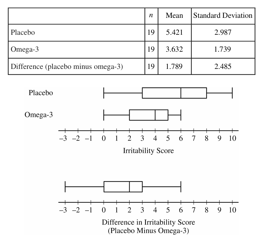
We need to perform a matched-pairs $t$-test for a population mean difference (\(\mu_d = \mu_{\text{placebo}} – \mu_{\text{omega-3}}\)). Our hypotheses are $H_0: \mu_d = 0$ versus $H_a: \mu_d > 0$. The conditions are met: treatments were randomly assigned, and the boxplot of the differences shows no extreme outliers or severe skewness, making the $t$-procedure appropriate for $n=19$.
Calculating the test statistic, we get $t = \frac{1.789 – 0}{2.485 / \sqrt{19}} \approx 3.138$ with $df = 18$. This yields a $p$-value of approximately $0.0028$.
Because the $p$-value ($0.0028$) is less than our significance level (\(\alpha = 0.05\)), we reject the null hypothesis. There is convincing statistical evidence to conclude that the omega-3 supplement decreases the true mean irritability score for patients with this medical condition.
Question

Most-appropriate topic codes (AP Statistics):
• Topic \(4.5\) — Carrying Out a Test for a Difference of Two Population Means (Part \( \mathrm{b} \))
▶️ Answer/Explanation
(a)
Yes, because the study used random assignment to assign participants to the two treatment groups.
Detailed Solution:
Random assignment creates comparable groups by balancing out potential confounding variables between the standard and new procedure groups.
Because of this design, a statistically significant difference in mean recovery times can indeed be attributed to the causal effect of the surgery type.
The inference applies to the population of patients similar to those who participated in the study.
(b)
Yes, the data provide convincing evidence that the new procedure results in lower average recovery time.
Detailed Solution:
We perform a two-sample $t$-test for a difference in means ($\mu_{standard} – \mu_{new} > 0$).
Calculating the standard error: $SE = \sqrt{\frac{34^2}{110} + \frac{29^2}{100}} = \sqrt{10.509 + 8.41} \approx 4.35$.
Calculating the $t$-statistic: $t = \frac{(217 – 186) – 0}{4.35} \approx 7.13$.
With a $t$-score of approximately $7.13$, the $p$-value is extremely small (virtually $0$), which is less than any standard significance level like $\alpha = 0.05$.
Therefore, we reject the null hypothesis and conclude there is overwhelming statistical evidence that the new procedure reduces recovery time.
Question
\(H_a : \mu > 122\)
Most-appropriate topic codes (AP Statistics):
• Topic \(4.5\) — Carrying Out a Test for a Population Mean (Part \( \mathrm{b} \))
• Topic \(4.7\) — Constructing a Confidence Interval for the Difference Between Two Population Means (Parts \( \mathrm{c} \), \( \mathrm{d} \), \( \mathrm{e} \))
▶️ Answer/Explanation
(a)
A Type II error occurs when the alternative hypothesis is actually true, but we fail to reject the null hypothesis.
In this context, a Type II error would occur if the true mean systolic blood pressure of all employees is greater than 122 mmHg, but the hypothesis test does not detect this — that is, the null hypothesis (\(H_0 : \mu = 122\)) is not rejected.
In plain terms: the employees really do have higher-than-national-average blood pressure, but the test fails to conclude so.
(b)
Since this is a one-sided (right-tailed) test with known \(\sigma\), we reject \(H_0\) when the test statistic exceeds the critical value \(z^* = 1.645\) at \(\alpha = 0.05\).
The test statistic is \(z = \dfrac{\bar{x} – \mu_0}{\sigma / \sqrt{n}} = \dfrac{\bar{x} – 122}{15/\sqrt{100}} = \dfrac{\bar{x} – 122}{1.5}\).
Setting \(\dfrac{\bar{x} – 122}{1.5} > 1.645\) and solving:
\(\bar{x} – 122 > 1.645 \times 1.5 = 2.4675\)
\(\boxed{\bar{x} > 124.4675 \text{ mmHg}}\)
Any sample mean greater than approximately 124.47 mmHg provides sufficient evidence to reject \(H_0\) at the \(\alpha = 0.05\) level.
(c)
Now the true population mean is \(\mu = 125\) mmHg (with \(\sigma = 15\), \(n = 100\)), so the sampling distribution of \(\bar{x}\) is approximately normal with mean 125 and standard deviation \(\dfrac{15}{\sqrt{100}} = 1.5\).
We want the probability that \(\bar{x}\) falls in the rejection region found in part (b):
\(P(\bar{x} > 124.4675) = P\!\left(z > \dfrac{124.4675 – 125}{1.5}\right) = P(z > -0.355)\ Folk\
\(\boxed{P(z > -0.355) \approx 0.64}\)
There is approximately a 64% probability that the null hypothesis will be rejected when the true mean is 125 mmHg.
(d)
The probability found in part (c) — the probability of correctly rejecting a false null hypothesis — is called the power of the test.
\(\boxed{\text{Power of the test} \approx 0.64}\)
(e)
The probability of rejecting \(H_0\) would be greater than 0.64 if the sample size is larger than 100.
A larger sample size \(n\) reduces the standard error of \(\bar{x}\): \(\sigma_{\bar{x}} = \dfrac{\sigma}{\sqrt{n}}\), so the sampling distribution becomes narrower.
This means the critical value \(\bar{x}^* = \mu_0 + z^* \cdot \dfrac{\sigma}{\sqrt{n}}\) would be smaller (closer to 122), lowering the threshold needed to reject \(H_0\).
With a lower rejection threshold, it becomes more likely that \(\bar{x}\) exceeds that threshold when the true mean is 125 mmHg — so the power of the test increases.
\(\boxed{\text{Probability of rejecting } H_0 \text{ would be greater than 0.64.}}\)
Question
Most-appropriate topic codes (AP Statistics):
• Topic \(4.5\) — Carrying Out a Test for a Population Mean Difference (full question)
▶️ Answer/Explanation
Step 1: State the hypotheses.
Let \(\mu_{\text{diff}}\) be the population mean difference in purchase price (woman − man) for identically equipped cars of the same model sold by the same dealer in the county.
\(H_0 : \mu_{\text{diff}} = 0\) (on average, women and men pay the same)
\(H_a : \mu_{\text{diff}} > 0\) (on average, women pay more than men)
Step 2: Identify the procedure and check conditions.
Since each pair consists of one man and one woman buying the same car model from the same dealer, the data are paired. The appropriate procedure is a paired \(t\)-test.
Random: The 8 car models were randomly selected and within each model, one man and one woman were randomly selected. The random condition is met.
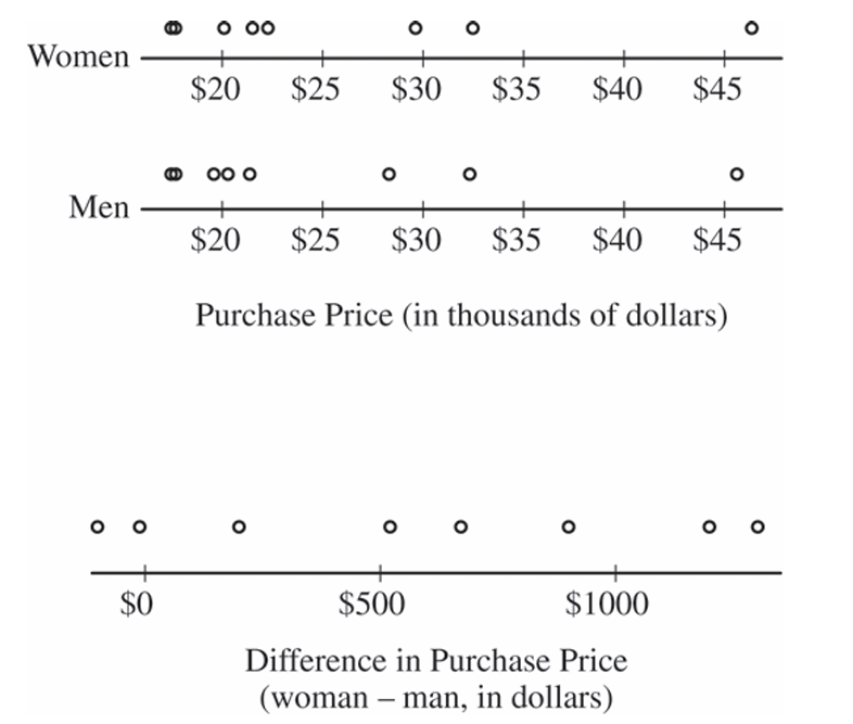
Normal/Large Sample: The sample size \(n = 8\) is small, so we cannot rely on the Central Limit Theorem. The dotplot of the differences shows a roughly symmetric distribution with no strong skewness or outliers, so it is reasonable to assume the population of differences is approximately normally distributed. The normal condition is considered met.
Step 3: Calculate the test statistic and \(p\)-value.
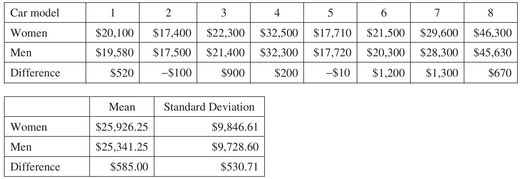
From the summary statistics for the differences: \(\bar{x}_d = 585\), \(s_d = 530.71\), \(n = 8\).
The test statistic is:
\(t = \dfrac{\bar{x}_d – 0}{\dfrac{s_d}{\sqrt{n}}} = \dfrac{585 – 0}{\dfrac{530.71}{\sqrt{8}}} = \dfrac{585}{187.63} \approx 3.12\)
Degrees of freedom: \(df = n – 1 = 8 – 1 = 7\)
The \(p\)-value for a one-sided \(t\)-test with \(t \approx 3.12\) and \(df = 7\) is:
\(p\text{-value} \approx 0.008\)
Step 4: State the conclusion in context.
Since the \(p\)-value of \(0.008\) is less than \(\alpha = 0.05\), we reject \(H_0\). The data provide convincing evidence that, on average, women pay more than men in the county for the same car model.
Question

Most-appropriate topic codes (AP Statistics):
• Topic \(4.5\) — Carrying Out a Test for a Population Mean or Population Mean Difference (Part \(\mathrm{a}\): test statistic, \(p\)-value, and conclusion)
• Topic \(2.3\) — Estimating Probabilities Using Simulation (Part \(\mathrm{b}\): simulation-based estimation of a \(p\)-value)
• Topic \(3.6\) — p-Values (Part \(\mathrm{b}\): interpreting simulated \(p\)-value evidence)
▶️ Answer/Explanation
(a)
Let \(\mu\) = the true mean number of fluid ounces dispensed into all juice bottles filled by the machine in the past hour.
Step 1 — Hypotheses:
\(H_0: \mu = 12.1\)
\(H_a: \mu \neq 12.1\)
Step 2 — Test: One-sample \(t\)-test for a mean (conditions are given as met; population standard deviation is unknown).
\(t = \frac{\bar{x} – \mu_0}{s/\sqrt{n}}\)
Step 3 — Mechanics:
Given: \(\bar{x} = 12.05\), \(s = 0.085\), \(n = 4\), \(\mu_0 = 12.1\)
\(t = \frac{12.05 – 12.1}{0.085/\sqrt{4}} = \frac{-0.05}{0.0425} \approx -1.176\)
Degrees of freedom: \(df = n – 1 = 3\)
Two-sided \(p\)-value:
\(p\text{-value} = 2 \cdot P(T_3 < -1.176) \approx 0.324\)
Step 4 — Conclusion:
Since the \(p\)-value of \(0.324\) is much larger than any reasonable significance level (such as \(\alpha = 0.05\)), we fail to reject \(H_0\).
There is not sufficient evidence to conclude that the mean amount of juice being dispensed is different from \(12.1\) fluid ounces. The machine does not need to be shut down on the basis of the mean.
(b)
In the simulation, 300 samples of size 4 were drawn from a normal population with \(\sigma = 0.05\). The sample standard deviation of \(s = 0.085\) from our actual data falls well out in the right tail of the dotplot.
Counting the dots at or beyond \(0.085\) in the dotplot, only about 12 out of 300 simulated values are as large or larger than \(0.085\).
This gives an estimated (simulated) \(p\)-value of:
\(\hat{p}\text{-value} = \frac{12}{300} = 0.04\)
Since this simulated \(p\)-value of \(0.04\) is less than \(\alpha = 0.05\), the sample does provide convincing evidence that the true standard deviation of the juice dispensed exceeds \(0.05\) fluid ounce. The machine should be shut down for recalibration.
Question
(b)
Most-appropriate topic codes (AP Statistics):
• Topic 4.5 — Carrying Out a Test for a Population Mean or Population Mean Difference (Part \(\mathrm{a}\))
• Topic 5.3 — Linear Regression Models (Part \(\mathrm{b}\))
• Topic 5.2 — Correlation (Part \(\mathrm{c}\))
• Topic 5.5 — Least-Squares Regression (Parts \(\mathrm{b}\), \(\mathrm{c}\), \(\mathrm{d}\))
▶️ Answer/Explanation
(a)
Step 1 — Hypotheses
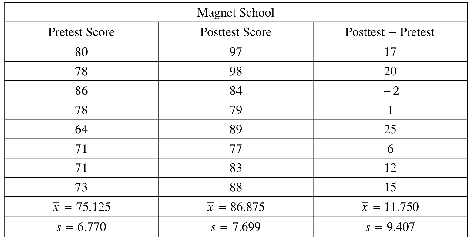
Let \(\mu_{\text{DiffM}}\) = the mean difference (posttest \(-\) pretest) for all students at the magnet school, and \(\mu_{\text{DiffO}}\) = the mean difference for all students who applied but were not selected and attended their original school.
\(H_0: \mu_{\text{DiffM}} = \mu_{\text{DiffO}}\)
\(H_a: \mu_{\text{DiffM}} > \mu_{\text{DiffO}}\)
Step 2 — Test and Conditions
We use a two-sample \(t\)-test for the difference of two means:
\(t = \dfrac{\bar{x}_M – \bar{x}_O}{\sqrt{\dfrac{s_M^2}{n_M} + \dfrac{s_O^2}{n_O}}}\)
- We need to assume randomness of the sampling used. It was stated in the stem that the students from the two different schools were randomly selected.
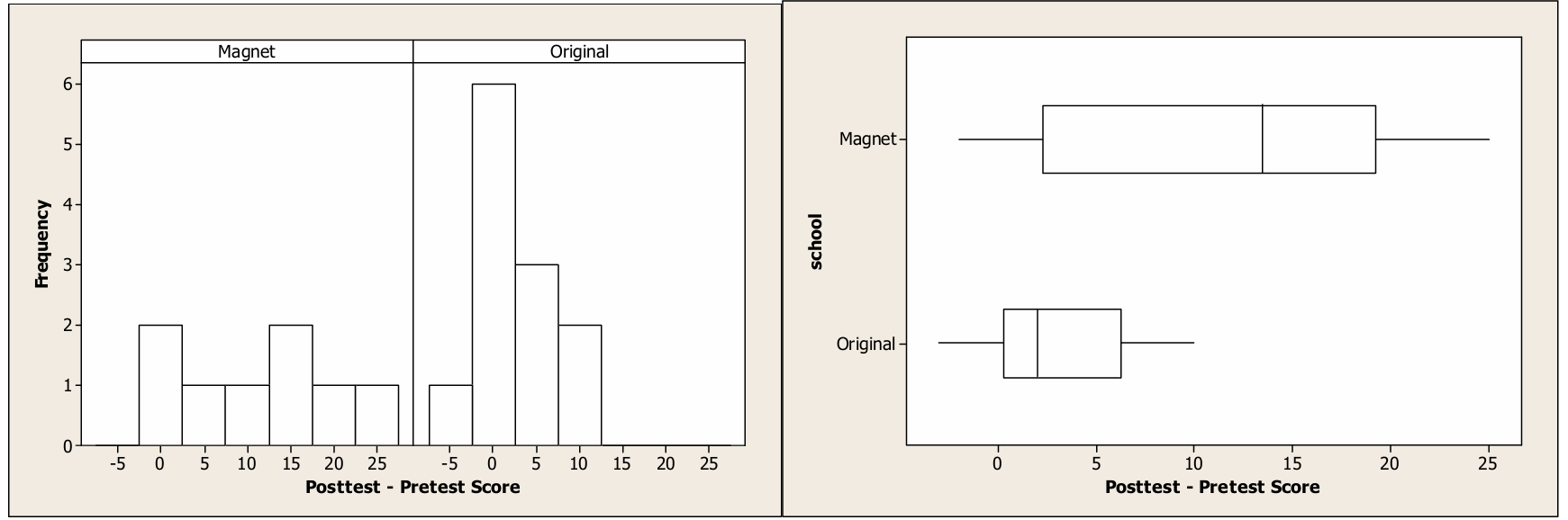
- We need to check the assumption that the distributions of differences (posttest – pretest) for each of the two schools are normally distributed. Based on histograms and boxplots of these differences, there are no outliers or extreme skewness. Because these graphs reveal no obvious departures from normality, it appears reasonable to proceed with the t-test.
Step 3 — Test Statistic and \(p\)-value
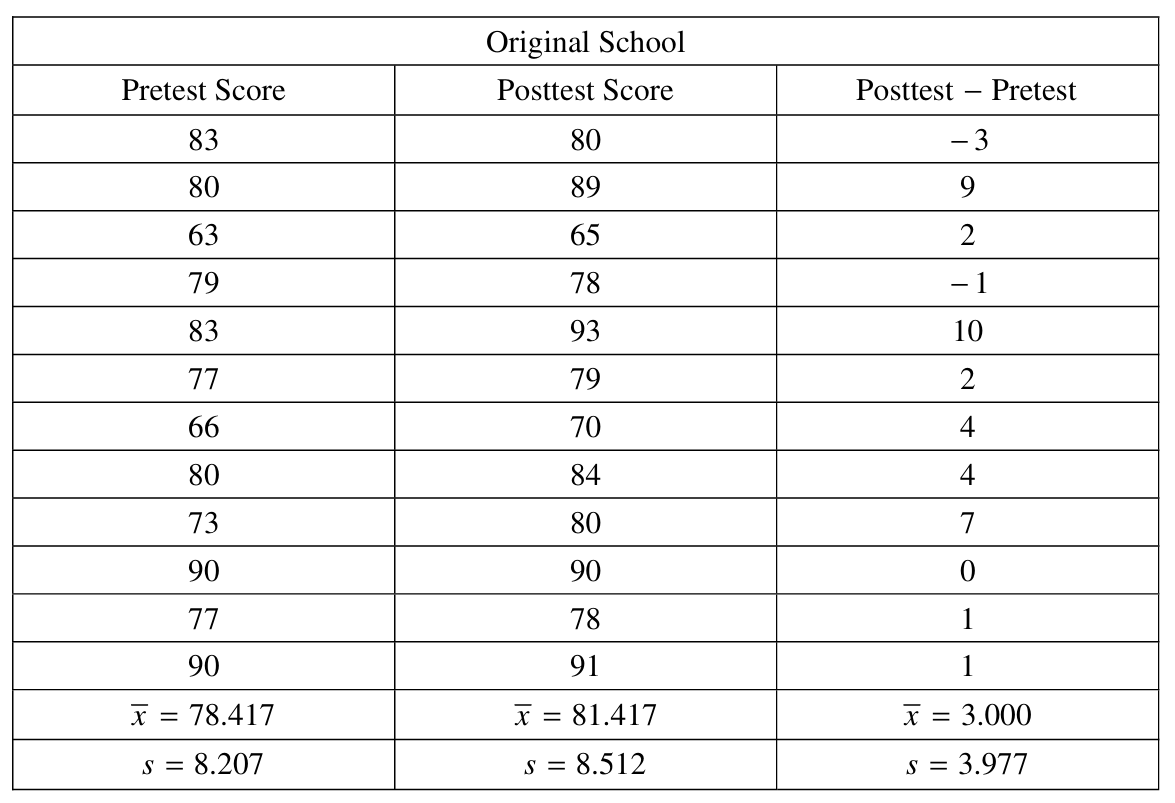
\(t = \dfrac{11.750 – 3.000}{\sqrt{\dfrac{(9.407)^2}{8} + \dfrac{(3.977)^2}{12}}} = \dfrac{8.750}{\sqrt{11.062 + 1.318}} = \dfrac{8.750}{\sqrt{12.380}} = \dfrac{8.750}{3.518} \approx 2.487\)
\(df \approx 8.69\), \(\quad p\text{-value} \approx 0.0177\)
Step 4 — Conclusion
Since \(p = 0.0177 < \alpha = 0.05\), we reject \(H_0\). There is convincing evidence that students who attend the magnet school have a higher mean improvement in science test scores than students who attended their original school.
(b)(i)
The regression equation for the magnet school is:
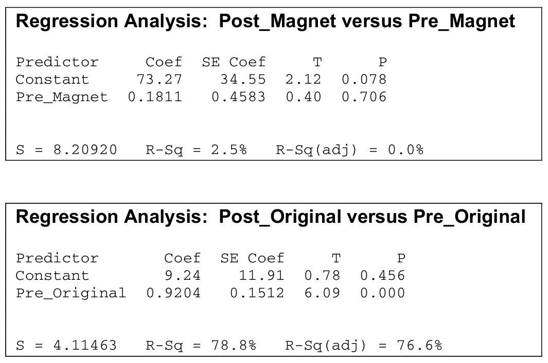
\(\hat{y} = 73.27 + 0.1811x\)
where \(x\) is the pretest score and \(\hat{y}\) is the predicted posttest score. The slope of \(0.1811\) means that for each additional point scored on the pretest by a magnet school student, the posttest score is predicted to increase by \(0.1811\) points, on average. The slope is positive but very close to zero, suggesting that pretest performance has almost no predictive power for posttest performance at the magnet school.
(b)(ii)
The regression equation for the original school is:
\(\hat{y} = 9.24 + 0.9204x\)
where \(x\) is the pretest score and \(\hat{y}\) is the predicted posttest score. The slope of \(0.9204\) means that for each additional point scored on the pretest by an original school student, the posttest score is predicted to increase by approximately \(0.9204\) points, on average — a nearly one-for-one relationship.
(c)(i) — Magnet School
From the regression output, the test statistic is \(t = 0.40\) with \(p\text{-value} = 0.706\).
Since \(0.706 > 0.05\), we fail to reject \(H_0\). There is insufficient evidence to conclude that there is a significant correlation between pretest score and posttest score at the magnet school. Pretest score is not a useful linear predictor of posttest score for magnet school students.
(c)(ii) — Original School
From the regression output, the test statistic is \(t = 6.09\) with \(p\text{-value} = 0.000\).
Since \(0.000 < 0.05\), we reject \(H_0\). There is strong evidence of a significant correlation between pretest score and posttest score at the original school. Pretest score is a very strong linear predictor of posttest score for original school students.
(d)
The two-sample \(t\)-test in part (a) told us only that the magnet school group had a higher average improvement — but it didn’t explain who benefited or by how much depending on their initial ability. The regression analyses reveal something much more interesting:
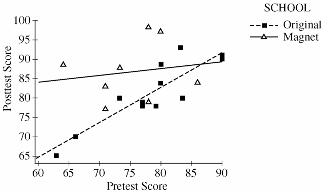
• At the magnet school, the slope is nearly zero (\(0.1811\)), and \(R^2 = 2.5\%\) — this means students score high on the posttest regardless of how they did on the pretest. A student who entered the magnet school with a low pretest score of 64 scored 89 on the posttest (an improvement of 25 points), while a student with a higher pretest score of 86 actually dropped 2 points. The magnet school appears to level the playing field and disproportionately benefits students who start with lower ability.
• At the original school, the slope is close to 1 (\(0.9204\)) and \(R^2 = 78.8\%\) — students essentially maintained their relative ranking, with high pretest scorers also achieving high posttest scores. There is very little “boost” effect for any student regardless of their starting point.
In short, the regression analyses reveal that the magnet school benefits students with low pretest scores the most, while the original school produces predictable but modest gains proportional to where students started.
Question
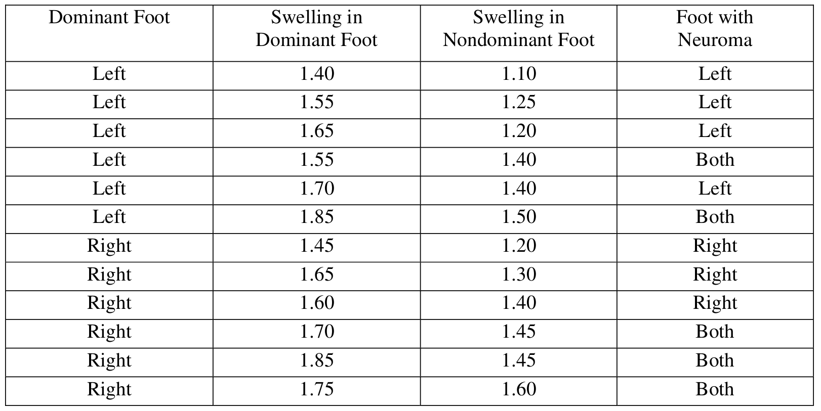
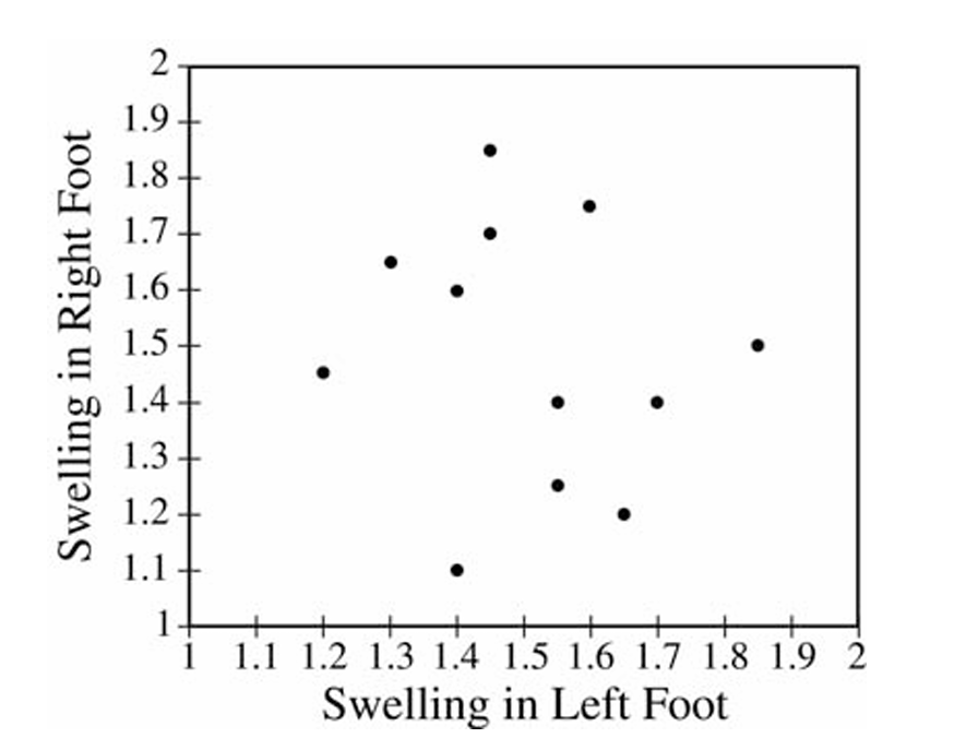
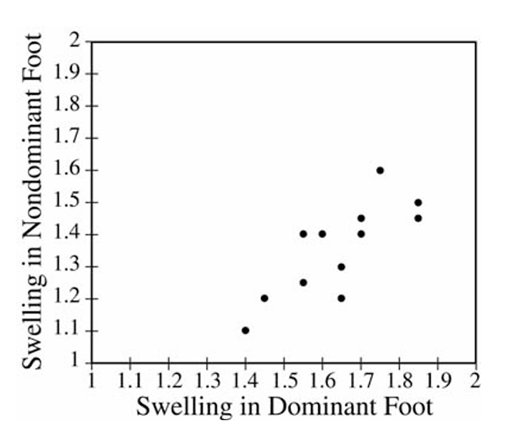
Most-appropriate topic codes (AP Statistics):
• Topic 4.4 — Setting Up a Test for a Population Mean or Population Mean Difference (Part \(\mathrm{c}\))
• Topic 4.5 — Carrying Out a Test for a Population Mean or Population Mean Difference (Part \(\mathrm{c}\))
• Topic 1.5 — Graphical Representations for One Quantitative Variable (Part \(\mathrm{d}\))
• Topic 1.9 — Comparisons of the Distributions for One Quantitative Variable (Part \(\mathrm{d}\))
▶️ Answer/Explanation
(a)
The trait that distinguishes the two groups in the scatterplot is the dominant foot (left or right). All the points in the upper-left cluster represent patients whose dominant foot is the right foot, while all the points in the lower-right cluster represent patients whose dominant foot is the left foot. The dominant foot type is the common trait, and it differs between the two groups.
(b)
Two conclusions become clear from this scatterplot that were not visible before:
First, there is a positive linear relationship between swelling in the dominant foot and swelling in the nondominant foot — as swelling in the dominant foot increases, swelling in the nondominant foot tends to increase as well.
Second, and importantly, every single point lies below the line \(y = x\), which means swelling in the dominant foot is consistently greater than swelling in the nondominant foot for all patients in the sample. This pattern across both groups combined is something you simply could not see in the left-foot vs. right-foot scatterplot from part (a).
(c)
We perform a matched-pairs \(t\)-test on the differences \(d_i = \text{(dominant swelling)} – \text{(nondominant swelling)}\).
The 12 differences are:
\(0.30,\ 0.30,\ 0.45,\ 0.15,\ 0.30,\ 0.35,\ 0.25,\ 0.35,\ 0.20,\ 0.25,\ 0.40,\ 0.15\)
State hypotheses (where \(\mu_d\) is the mean difference, dominant minus nondominant):
\(H_0: \mu_d = 0\)
\(H_a: \mu_d \neq 0\)
Check conditions:
1. We are told a random sample was selected from the population of adult females with Morton’s neuroma.
2. A dotplot of the differences shows a roughly symmetric, unimodal distribution with no outliers — it is reasonable to treat the population of differences as approximately normal.
Compute the test statistic:
\(\bar{x}_d = 0.2875, \quad s_d = 0.0932, \quad n = 12, \quad df = 11\)
\(t = \dfrac{\bar{x}_d – 0}{\dfrac{s_d}{\sqrt{n}}} = \dfrac{0.2875 – 0}{\dfrac{0.0932}{\sqrt{12}}} = 10.68\)
\(p\text{-value} \approx 0.0000004 \approx 0\)
Since the \(p\)-value is essentially \(0\), which is far less than any reasonable significance level \(\alpha\), we reject \(H_0\). There is very convincing statistical evidence that the mean swelling in the dominant foot is different from (and specifically greater than) the mean swelling in the nondominant foot for adult females who have Morton’s neuroma in at least one foot.
(d)
To suggest a diagnostic criterion, we separate all 24 swelling measurements into two groups: the 17 foot measurements from feet that have Morton’s neuroma and the 7 foot measurements from feet that do not have Morton’s neuroma. A stacked dotplot of the two groups is shown below: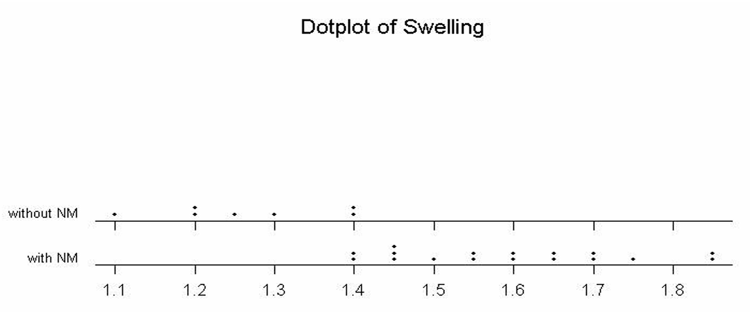
The dotplot makes it visually clear that all 7 feet without Morton’s neuroma have swelling measurements of \(1.40\) or below, while the feet with Morton’s neuroma have swelling values of \(1.40\) and above (with the measurements extending up to \(1.85\)). Based on this graphical display, a reasonable diagnostic criterion is:
\(\boxed{\text{Swelling measurement} \geq 1.4 \Rightarrow \text{diagnose Morton’s neuroma}}\)
A cutoff of approximately \(1.4\) or higher serves as a sensible threshold for diagnosing Morton’s neuroma, since it cleanly separates the feet with and without the condition in this dataset.
Question

Most-appropriate topic codes (AP Statistics):
• Topic 4.5 — Carrying Out a Test for a Population Mean or Population Mean Difference (Test Mechanics and Conclusion)
• Topic 1.5 — Graphical Representations for One Quantitative Variable (Checking the Distribution of Differences)
▶️ Answer/Explanation
We conduct a paired \(t\)-test for the mean difference in the level of E. coli bacteria contamination detected by the two methods.
Step 1 — Hypotheses
Let \(\mu_d\) be the population mean difference in E. coli contamination levels (Method A \(-\) Method B).
\(H_0: \mu_d = 0\) (no difference in mean contamination detected by the two methods)
\(H_a: \mu_d \neq 0\) (there is a difference in mean contamination detected by the two methods)
Step 2 — Identify Test and Check Conditions
We use a paired \(t\)-test with test statistic:
\(t = \dfrac{\bar{x}_d – 0}{s_d / \sqrt{n_d}}\)
First, compute the differences \(d_i = A_i – B_i\) for each specimen:
\(-0.3,\quad 0.5,\quad 0.3,\quad 0.6,\quad 0.8,\quad 0.7,\quad 1.2,\quad 0.2,\quad -0.1,\quad -1.0\)
Condition 1 — Independence: The 10 specimens were randomly selected, so it is reasonable to assume the 10 pairs of measurements are independent of one another.
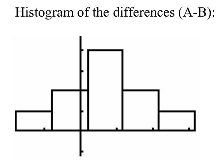
Condition 2 — Normality of Differences: With only \(n = 10\) differences, we check a histogram or boxplot of the differences. The histogram of the differences \((A – B)\) is roughly symmetric with no apparent outliers, so it is reasonable to assume the population distribution of differences is approximately normal.
Step 3 — Mechanics
From the differences:
\(\bar{x}_d = 0.29, \qquad s_d = 0.6297, \qquad n = 10\)
\(t = \dfrac{0.29 – 0}{0.6297/\sqrt{10}} = \dfrac{0.29}{0.1991} \approx 1.456\)
\(\text{degrees of freedom} = n – 1 = 9\)
\(p\text{-value} = 2 \times P(t_9 > 1.456) \approx 0.1793\)
Step 4 — Conclusion
Since the \(p\)-value of \(0.1793\) is greater than \(\alpha = 0.05\), we fail to reject \(H_0\).
We do not have statistically significant evidence to conclude that there is a difference in the mean amount of E. coli bacteria detected by the two methods for this type of beef.
\(\boxed{p\text{-value} = 0.1793 > 0.05 \Rightarrow \text{Fail to reject } H_0; \text{ no significant difference between the two methods.}}\)
Question

Most-appropriate topic codes (AP Statistics):
• Topic 4.5 — Carrying Out a Test for a Population Mean or Population Mean Difference (Parts \(\mathrm{b}\), \(\mathrm{c}\), \(\mathrm{d}\))
• Topic 2.12 — Sampling Distributions and the Central Limit Theorem (Parts \(\mathrm{e}\), \(\mathrm{f}\))
▶️ Answer/Explanation
(a)
Let \(\sigma^2\) denote the true population variance of the readings of recently manufactured thermostats (in degrees Fahrenheit squared).
\(H_0: \sigma^2 = 1.52 \qquad \text{(variance has not changed)}\)
\(H_a: \sigma^2 > 1.52 \qquad \text{(recently produced thermostats are more variable)}\)
(b)
First, compute the sample standard deviation from the 10 readings:
\(s^2 = 2.0383 \implies s = 1.4277\)
Then compute the test statistic:
\(\chi^2 = \frac{(n-1)s^2}{1.52} = \frac{9 \times 2.0383}{1.52} = \frac{18.345}{1.52}\)
\(\boxed{\chi^2 \approx 12.069}\)
(c)
Under \(H_0\), the test statistic follows a \(\chi^2\) distribution with \(n – 1 = 9\) degrees of freedom.
The \(p\)-value is the probability of obtaining a test statistic as large as or larger than the observed value:
\(p\text{-value} = P\!\left(\chi^2_9 \geq 12.069\right) \approx 0.2094\)
(From the table: \(0.20 < p\text{-value} < 0.25\))
Since the \(p\)-value \(\approx 0.2094 > 0.05\), we fail to reject \(H_0\). There is not statistically significant evidence at the \(\alpha = 0.05\) level that the recently manufactured thermostats have become more variable than in the past.
\(\boxed{\text{Fail to reject } H_0;\ p\text{-value} \approx 0.209}\)
(d)
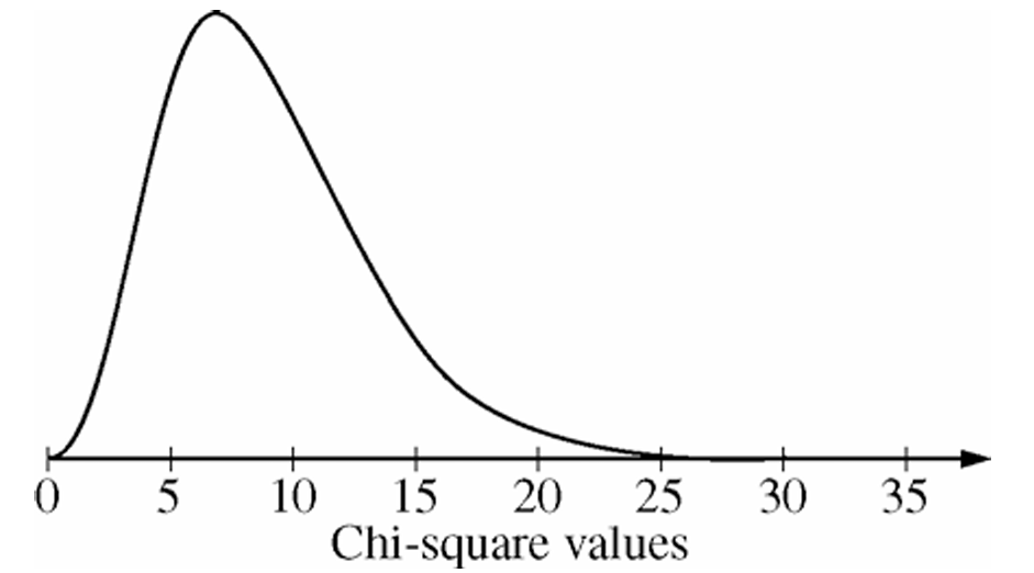
The smallest value of the test statistic that leads to rejection of \(H_0\) at the 5% significance level is the 95th percentile of the \(\chi^2\) distribution with 9 degrees of freedom:
\(\boxed{\chi^2_{0.05,\,9} = 16.92}\)
The rejection region consists of all chi-square values greater than or equal to \(16.92\), which corresponds to the shaded right tail of the \(\chi^2_9\) curve (as marked on the graph above).
(e)
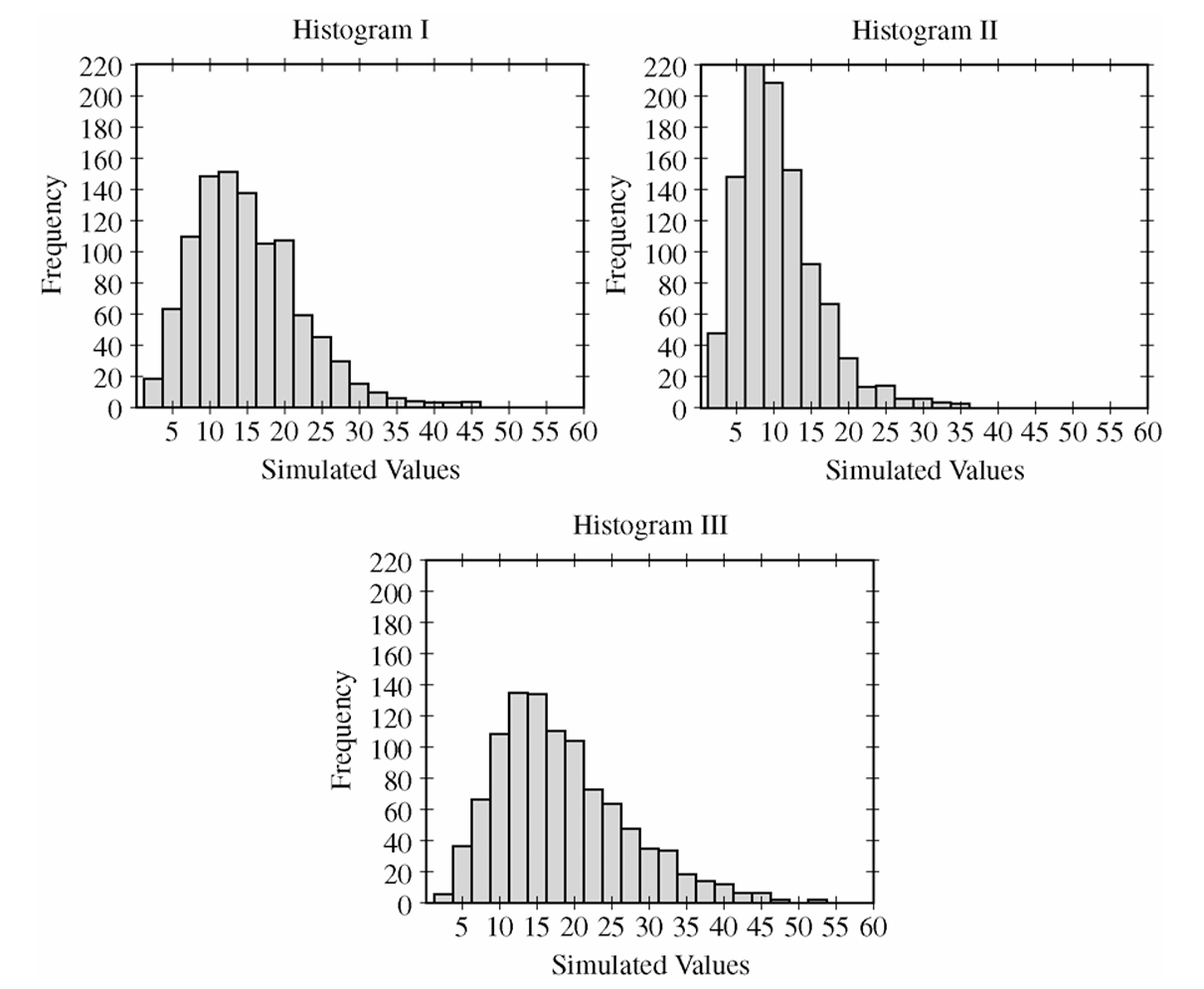
The rejection region — all simulated values to the right of \(16.92\) — should be marked on each of the three histograms (Histogram I, Histogram II, and Histogram III) as indicated by the dashed vertical lines in the diagrams above.
(f)
Largest variance → Histogram III. A population with a larger variance will tend to produce larger sample variances \(s^2\), and hence larger values of the test statistic \(\frac{(n-1)s^2}{1.52}\). Histogram III has the greatest proportion of simulated values falling to the right of \(16.92\) — meaning it has the highest probability of correctly rejecting \(H_0\) — so it corresponds to the population with the largest variance.
Smallest variance → Histogram II. Histogram II has its simulated values concentrated most tightly at smaller values, with the smallest proportion of values exceeding \(16.92\). This means it has the lowest probability of rejecting \(H_0\), consistent with coming from the population whose variance is smallest (and closest to \(1.52\) among the three).
\(\boxed{\text{Largest variance: Histogram III} \qquad \text{Smallest variance: Histogram II}}\)
Question
Most-appropriate topic codes (AP Statistics):
• Topic 4.5 — Carrying Out a Test for a Population Mean or Population Mean Difference (Test Statistic, \(p\)-value, and Conclusion)
▶️ Answer/Explanation
Step 1: State the hypotheses.
Let \(\mu_D\) denote the mean difference (after \(-\) before) in dexterity scores for the population of individuals enrolled in the program.
\(H_0: \mu_D = 0\)
\(H_a: \mu_D > 0\)
Step 2: Identify the correct test and check conditions.
Since the data consist of before-and-after measurements on the same individuals, we use a one-sample paired \(t\)-test on the differences \(d_i = \text{after}_i – \text{before}_i\).
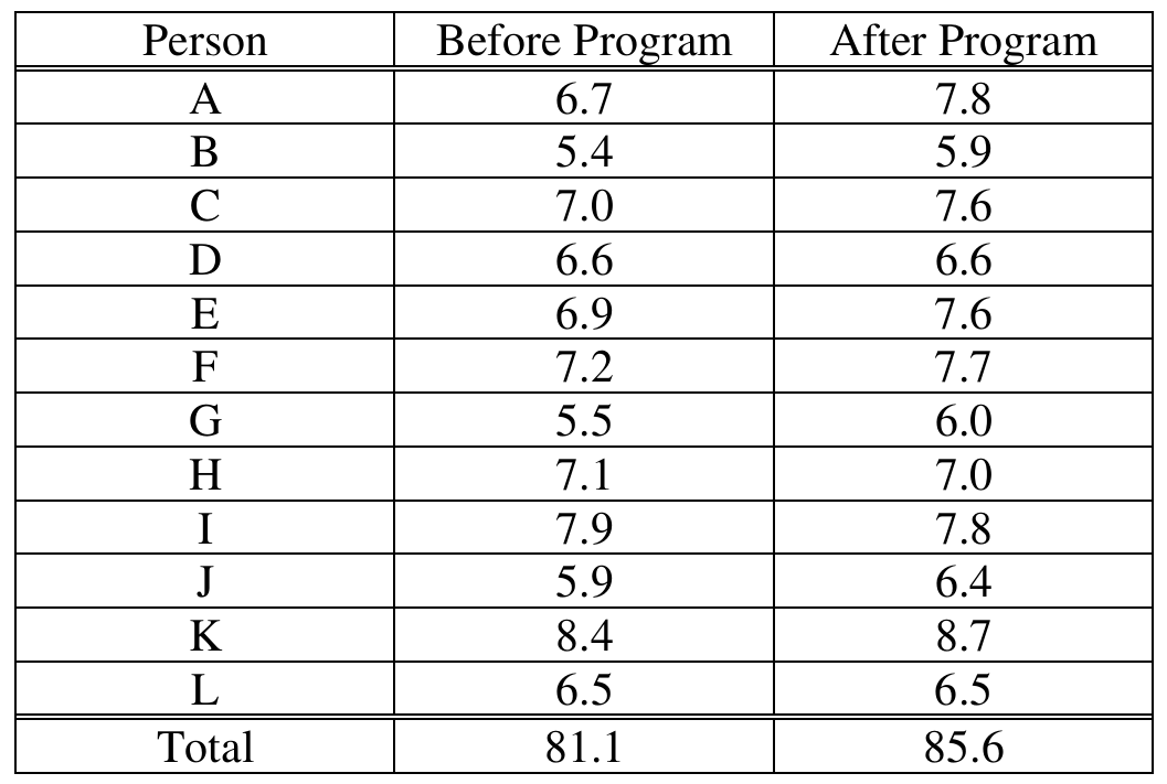
The individual differences are: \(1.1,\ 0.5,\ 0.6,\ 0,\ 0.7,\ 0.5,\ 0.5,\ -0.1,\ -0.1,\ 0.5,\ 0.3,\ 0\)
Conditions:
1. Random sample: The problem states that the 12 people are a random sample from the population enrolled in the program.
2. Approximate normality: With only \(n = 12\) observations, we check the distribution of differences. A dotplot or histogram of the differences shows no strong skewness or outliers, so it is reasonable to assume the differences are approximately normally distributed.
Step 3: Compute the test statistic and \(p\)-value.
From the differences, we compute:
\(\bar{d} = \frac{85.6 – 81.1}{12} = \frac{4.5}{12} = 0.375\)
\(s_d = 0.367\)
\(\text{Degrees of freedom} = n – 1 = 12 – 1 = 11\)
\(t = \frac{\bar{d} – 0}{s_d / \sqrt{n}} = \frac{0.375 – 0}{0.367 / \sqrt{12}} = \frac{0.375}{0.1059} = 3.54\)
\(p\text{-value} = P(t_{11} > 3.54) \approx 0.002\)
Step 4: State the conclusion in context.
Since the \(p\)-value (\(\approx 0.002\)) is less than any common significance level such as \(\alpha = 0.05\), we reject \(H_0\).
There is sufficient, statistically significant evidence to conclude that, on average, people who completed the 6-week training program have meaningfully increased their manual dexterity.
\(\boxed{t = 3.54,\quad p\text{-value} \approx 0.002 \implies \text{Reject } H_0 \text{ — mean dexterity has significantly increased}}\)
Question
| Sample | Minimum | Sample | Minimum | Sample | Minimum |
| 1 | 121.45 | 51 | 124.28 | 101 | 125.25 |
| 2 | 122.51 | 52 | 124.29 | 102 | 125.31 |
| 3 | 122.53 | 53 | 124.30 | 103 | 125.36 |
| 4 | 122.72 | 54 | 124.31 | 104 | 125.38 |
| 5 | 122.75 | 55 | 124.34 | 105 | 125.40 |
| 6 | 122.89 | 56 | 124.36 | 106 | 125.42 |
| 7 | 122.93 | 57 | 124.37 | 107 | 125.48 |
| 8 | 122.99 | 58 | 124.37 | 108 | 125.49 |
| 9 | 123.04 | 59 | 124.39 | 109 | 125.50 |
| 10 | 123.08 | 60 | 124.39 | 110 | 125.52 |
| 11 | 123.09 | 61 | 124.41 | 111 | 125.54 |
| 12 | 123.10 | 62 | 124.44 | 112 | 125.56 |
| 13 | 123.31 | 63 | 124.53 | 113 | 125.61 |
| 14 | 123.34 | 64 | 124.53 | 114 | 125.67 |
| 15 | 123.39 | 65 | 124.54 | 115 | 125.72 |
| 16 | 123.40 | 66 | 124.55 | 116 | 125.76 |
| 17 | 123.41 | 67 | 124.55 | 117 | 125.77 |
| 18 | 123.41 | 68 | 124.55 | 118 | 125.78 |
| 19 | 123.46 | 69 | 124.55 | 119 | 125.79 |
| 20 | 123.49 | 70 | 124.58 | 120 | 125.84 |
| 21 | 123.51 | 71 | 124.67 | 121 | 125.87 |
| 22 | 123.57 | 72 | 124.69 | 122 | 125.87 |
| 23 | 123.58 | 73 | 124.73 | 123 | 125.90 |
| 24 | 123.59 | 74 | 124.77 | 124 | 125.90 |
| 25 | 123.60 | 75 | 124.78 | 125 | 125.93 |
| 26 | 123.66 | 76 | 124.78 | 126 | 125.93 |
| 27 | 123.67 | 77 | 124.80 | 127 | 125.93 |
| 28 | 123.72 | 78 | 124.80 | 128 | 125.94 |
| 29 | 123.75 | 79 | 124.81 | 129 | 125.98 |
| 30 | 123.77 | 80 | 124.85 | 130 | 126.00 |
| 31 | 123.78 | 81 | 124.91 | 131 | 126.03 |
| 32 | 123.84 | 82 | 124.92 | 132 | 126.05 |
| 33 | 123.91 | 83 | 124.92 | 133 | 126.05 |
| 34 | 123.93 | 84 | 124.96 | 134 | 126.06 |
| 35 | 123.95 | 85 | 125.00 | 135 | 126.09 |
| 36 | 123.95 | 86 | 125.01 | 136 | 126.15 |
| 37 | 123.98 | 87 | 125.02 | 137 | 126.15 |
| 38 | 123.99 | 88 | 125.02 | 138 | 126.16 |
| 39 | 124.05 | 89 | 125.03 | 139 | 126.19 |
| 40 | 124.05 | 90 | 125.04 | 140 | 126.19 |
| 41 | 124.06 | 91 | 125.05 | 141 | 126.25 |
| 42 | 124.12 | 92 | 125.07 | 142 | 126.26 |
| 43 | 124.14 | 93 | 125.08 | 143 | 126.33 |
| 44 | 124.15 | 94 | 125.09 | 144 | 126.35 |
| 45 | 124.16 | 95 | 125.14 | 145 | 126.45 |
| 46 | 124.19 | 96 | 125.18 | 146 | 126.50 |
| 47 | 124.23 | 97 | 125.21 | 147 | 126.57 |
| 48 | 124.27 | 98 | 125.21 | 148 | 126.62 |
| 49 | 124.28 | 99 | 125.22 | 149 | 126.64 |
| 50 | 124.28 | 100 | 125.25 | 150 | 126.95 |
Most-appropriate topic codes (AP Statistics):
• Topic 4.5 — Carrying Out a Test for a Population Mean or Population Mean Difference (Part a)
• Topic 2.11 — The Normal Distribution (Parts b, c)
• Topic 2.3 — Estimating Probabilities Using Simulation (Part d)
▶️ Answer/Explanation
(a)
Step 1 — State the hypotheses:
\( H_0: \mu = 128 \text{ fl oz} \quad \text{vs.} \quad H_a: \mu < 128 \text{ fl oz} \)
where \(\mu\) is the true mean amount of milk in containers from this plant.
We test whether the mean is below 128 fl oz, since that would indicate non-compliance.
Step 2 — Identify the procedure and check conditions:
Use a one-sample \(t\)-test for a mean:
\( t = \frac{\bar{x} – \mu_0}{s/\sqrt{n}} \)
The problem states the filling process produces a normal distribution, so the normality condition is satisfied.
The containers were randomly sampled, so independence holds.
Step 3 — Compute the test statistic and p-value:
With \(\bar{x} = 127.2\), \(\mu_0 = 128\), \(s = 2.1\), \(n = 12\):
\( t = \frac{127.2 – 128}{2.1/\sqrt{12}} = \frac{-0.8}{0.6062} \approx -1.319 \)
Degrees of freedom: \(df = n – 1 = 11\).
For a one-tailed test with \(t = -1.319\) and \(df = 11\):
\( p\text{-value} = P(T_{11} < -1.319) \approx 0.107 \)
Step 4 — State the conclusion in context:
Since the p-value of \(0.107\) is greater than any reasonable significance level (e.g., \(\alpha = 0.05\)), we fail to reject \(H_0\). There is not sufficient evidence to conclude that the plant is out of compliance. The sample mean of 127.2 fl oz is below 128, but the difference is small enough that it could plausibly be due to random sampling variability alone.
(b)
Let \(X\) be the amount of milk in a randomly selected container, where \(X \sim N(128.0,\ 2.0)\). We want \(P(X \geq 125)\).
Standardize by converting to a \(z\)-score: \( z = \frac{125 – 128}{2} = \frac{-3}{2} = -1.5 \)
Using the standard normal table:
\( P(X \geq 125) = P(Z \geq -1.5) = 1 – P(Z < -1.5) = 1 – 0.0668 \)
\( \boxed{P(X \geq 125) = 0.9332} \)
So about 93.3% of containers from this machine will contain at least 125 fl oz.
(c)
Let \(X_{(1)} = \min(X_1, X_2, \ldots, X_{12})\) be the smallest value among 12 randomly selected containers.
For the minimum to be at least 125 fl oz, every single one of the 12 containers must contain at least 125 fl oz.
Since the containers are independent:
\( P(X_{(1)} \geq 125) = P(X_1 \geq 125) \times P(X_2 \geq 125) \times \cdots \times P(X_{12} \geq 125) \)
\( = [P(X \geq 125)]^{12} = (0.9332)^{12} \)
\( \boxed{P(X_{(1)} \geq 125) \approx 0.4362} \)
There is roughly a 43.6% chance that the smallest of 12 containers all meet the 125 fl oz threshold.
Even though each individual container has a 93.3% chance of passing, the probability that all 12 pass simultaneously drops considerably.
(d)
From the sorted list of 150 simulated minimums, we count how many are at least 125 fl oz. Scanning the table, the minimums first reach 125.00 at sample 85. From sample 85 through sample 150, that gives:
\( 150 – 85 + 1 = 66 \text{ minimums that are} \geq 125 \text{ fl oz} \)
The simulated probability estimate is therefore:
\( \hat{p} = \frac{66}{150} \approx \boxed{0.44} \)
Comparison with the theoretical value:
The theoretical probability from part (c) was \(0.4362\).
The simulation estimate of \(0.44\) is very close — the difference is only:
\( |0.44 – 0.4362| = 0.0038 \)
This is a tiny discrepancy, which is exactly what we expect from a simulation of this size.
The simulation does an excellent job of approximating the true theoretical probability, confirming that the independence-based calculation in part (c) is correct.
Question
Most-appropriate topic codes (AP Statistics):
• Topic 4.4 — Setting Up a Test for a Population Mean or Population Mean Difference (Part b)
• Topic 4.5 — Carrying Out a Test for a Population Mean or Population Mean Difference (Part b)
• Topic 4.2 — Constructing a Confidence Interval for a Population Mean or Population Mean Difference (Part c)
• Topic 4.3 — Justifying a Claim Based on a Confidence Interval for a Population Mean or Population Mean Difference (Parts c, d)
▶️ Answer/Explanation
(a)
The appropriate procedure is a one-sample \(t\)-interval for the population mean \(\mu\).
Conditions:
— The data come from a random sample of 50 people.
— \(\sigma\) is unknown; using the sample standard deviation \(s = 15\).
— \(n = 50 \geq 30\), so by the Central Limit Theorem the sampling distribution of \(\bar{x}\) is approximately normal.
Given: \(\bar{x} = 24\), \(s = 15\), \(n = 50\), and \(df = 49\). For a 95% confidence interval, \(t^* \approx 2.009\) (using \(df = 49\)).
The confidence interval formula is:
\(\bar{x} \pm t^* \cdot \dfrac{s}{\sqrt{n}}\)
\(24 \pm 2.009 \cdot \dfrac{15}{\sqrt{50}}\)
\(24 \pm 2.009 \times 2.121\)
\(24 \pm 4.262\)
\(\boxed{(19.738,\ 28.262) \text{ mg/dl}}\)
Interpretation: We are 95% confident that the true population mean reduction in cholesterol level after one month of use of the new drug is between approximately 19.7 mg/dl and 28.3 mg/dl.
(b)
The confidence interval and the hypothesis test led to different conclusions because they are based on different types of procedures that correspond to different questions being asked.
The 95% two-sided confidence interval is equivalent to a two-sided hypothesis test at \(\alpha = 0.05\). The two-sided \(p\)-value for testing \(H_0: \mu = 20\) against \(H_a: \mu \neq 20\) would be \(2 \times 0.033 = 0.066\), which exceeds \(\alpha = 0.05\) — hence the confidence interval (which captures values consistent with a two-sided test) includes 20 and fails to reject \(H_0\) at the 0.05 level.
The hypothesis test, however, is one-sided (\(H_a: \mu > 20\)) with a one-sided \(p\)-value of \(0.033 < 0.05\), which leads to rejecting \(H_0\). A one-sided test is more powerful in the direction specified and uses only one tail of the distribution. The two procedures are therefore testing different things, and it is the mismatch — using a two-sided interval to evaluate a one-sided hypothesis — that creates the apparent contradiction in conclusions.
\(\boxed{\text{Two-sided CI} \leftrightarrow \text{two-sided test (}p = 0.066 > 0.05\text{)}; \quad \text{one-sided test: }p = 0.033 < 0.05}\)
(c)
For a one-sided 95% confidence interval, we need to find \(t^*\) such that 95% of the \(t\)-distribution with \(df = 49\) lies above \(-t^*\) (i.e., only one tail of area 0.05).
This corresponds to a tail probability of \(p = 0.05\) (one tail) with \(df = 49\). From the \(t\)-table:
\(\boxed{t^* = 1.676 \quad (df = 49,\ \text{one tail}, \ \alpha = 0.05)}\)
Now compute \(L\):
\(L = \bar{x} – t^* \cdot \dfrac{s}{\sqrt{n}} = 24 – 1.676 \cdot \dfrac{15}{\sqrt{50}}\)
\(= 24 – 1.676 \times 2.121\)
\(= 24 – 3.555\)
\(\boxed{L \approx 20.4 \text{ mg/dl}}\)
Interpretation: We are 95% confident that the true mean reduction in cholesterol level after one month of use of the new drug is greater than approximately 20.4 mg/dl.
(d)
Yes, the regulatory agency would have reached a different conclusion using the one-sided confidence interval. The one-sided interval shows that the agency can be 95% confident that the true mean reduction is greater than \(L \approx 20.4\) mg/dl, which is already above the threshold of 20 mg/dl required for recommendation. Since the entire range of plausible values for \(\mu\) under the one-sided interval lies above 20, the agency would have had convincing evidence that the new drug reduces cholesterol by more than 20 mg/dl on average — and would therefore have recommended the drug for use.
\(\boxed{L \approx 20.4 > 20 \Rightarrow \text{Yes, different conclusion: agency would recommend the drug}}\)