
AP Statistics 4.8 Justifying a Claim Based on a Confidence Interval for the Difference Between Two Population Means- Exam Style Questions - FRQs - New Syllabus
Question
Most-appropriate topic codes (AP Statistics):
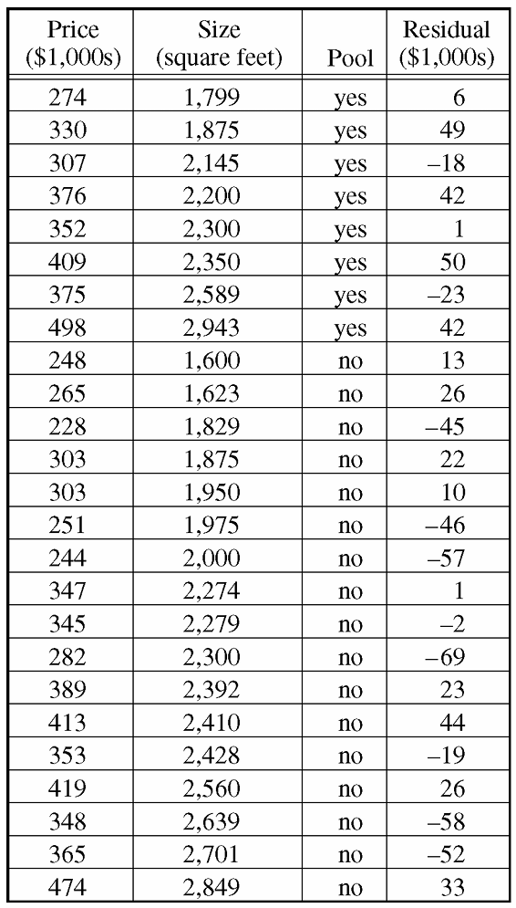
• Topic \(5.4\) — Residuals (Parts \(\mathrm{b}\), \(\mathrm{c}\))
• Topic \(5.5\) — Least-Squares Regression (Parts \(\mathrm{a}\), \(\mathrm{b}\), \(\mathrm{c}\), \(\mathrm{e}\))
• Topic \(4.8\) — Justifying a Claim Based on a Confidence Interval for the Difference Between Two Population Means (Part \(\mathrm{d}\))
▶️ Answer/Explanation
(a)
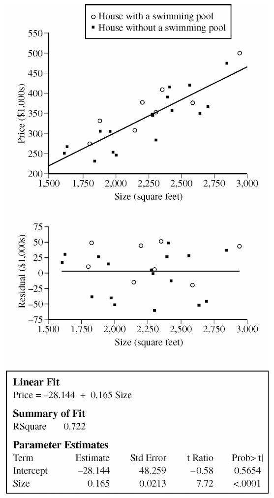
The slope of the least squares regression line is \(0.165\) (in thousands of dollars per square foot).
In context: for each additional square foot of house size, the predicted price of the house increases by \(0.165\) thousand dollars, or \$165, on average.
The slope tells us the rate at which the model expects price to grow with size — not a guarantee for any individual house, but the average trend across houses in this part of the city.
(b)
The residual value of 49 for this house indicates that its actual price is 49 thousand dollars higher than the model would predict for a house of its size.
(c)
We estimate the pool premium by comparing the average residuals of the two groups. If a group’s residuals average positive, the model consistently underestimates their prices; if negative, it overestimates.
Houses with a swimming pool (8 houses, residuals: \(6, 49, -18, 42, 1, 50, -23, 42\)):
\(\bar{e}_{\text{pool}} = \frac{6 + 49 + (-18) + 42 + 1 + 50 + (-23) + 42}{8} = \frac{149}{8} = 18.625 \text{ thousand dollars}\)
Houses without a swimming pool (17 houses, residuals: \(13, 26, -45, 22, 10, -46, -57, 1, -2, -69, 23, 44, -19, 26, -58, -52, 33\)):
\(\bar{e}_{\text{no pool}} = \frac{13 + 26 + (-45) + 22 + 10 + (-46) + (-57) + 1 + (-2) + (-69) + 23 + 44 + (-19) + 26 + (-58) + (-52) + 33}{17} = \frac{-150}{17} \approx -8.824 \text{ thousand dollars}\)
The estimated price premium for a swimming pool is the difference between these two averages:
\(\bar{e}_{\text{pool}} – \bar{e}_{\text{no pool}} = 18.625 – (-8.824) = \boxed{27.4 \text{ thousand dollars}}\)
This tells us that, for two houses of the same size, the one with a swimming pool is estimated to cost about \$27,400 more. The logic: pool houses have residuals that average \$18,625 above the model’s predictions, while no-pool houses sit \$8,824 below — that gap reflects the pool’s unmodeled contribution to price.
(d)
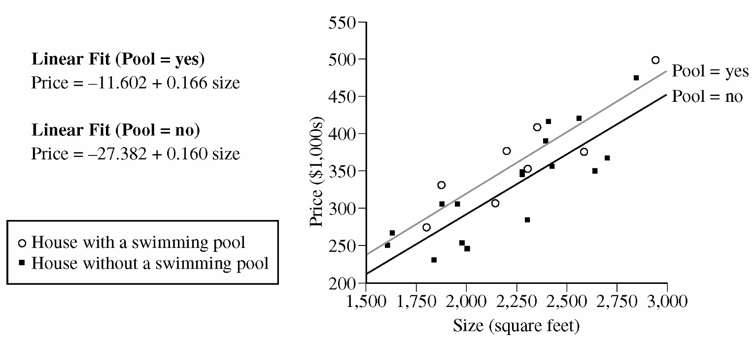
The 95% confidence interval for the true difference in slopes is \((-0.099,\ 0.110)\).
Since this interval contains zero, we cannot conclude there is a statistically significant difference between the two slopes at the 5% significance level. Zero is a plausible value for the true difference, which means it is entirely possible that the two population regression lines have the same slope.
In practical terms: the rate at which price increases with size appears to be the same for pool homes and non-pool homes — a pool shifts the price up by a roughly constant amount, but doesn’t change how sensitive the price is to square footage.
(e)
Since the two slopes are not significantly different, we pick a house size within the data range — say, \(\text{size} = 2{,}250\) sq ft (near the center of the distribution) — and compare predicted prices from both models.
Predicted price with pool:
\(\widehat{\text{Price}}_{\text{pool}} = -11.602 + 0.166 \times 2250 = -11.602 + 373.500 = 361.898 \text{ thousand dollars}\)
Predicted price without pool:
\(\widehat{\text{Price}}_{\text{no pool}} = -27.382 + 0.160 \times 2250 = -27.382 + 360.000 = 332.618 \text{ thousand dollars}\)
Estimated price premium for a pool:
\(361.898 – 332.618 = \boxed{29.280 \text{ thousand dollars} \approx \$29{,}280}\)
Comparison with part (c): The estimate from part (e), approximately \$29,280, is quite similar to the \$27,400 estimate obtained in part (c) from the residual averages. Both methods point to a pool adding roughly \$27,000–\$29,000 to the price of a house, giving us confidence that this is a reasonable estimate of the pool’s effect regardless of which approach we use.
Note — Alternative approach (difference in intercepts): Because the slopes were found not to be significantly different, we can also subtract the two fitted equations directly:
\((-11.602 + 0.166 \cdot x) – (-27.382 + 0.160 \cdot x) = 15.780 + 0.006 \cdot x\)
This gives the price difference as a function of size. For \(x = 2250\): \(15.780 + 0.006 \times 2250 = 15.780 + 13.500 = 29.280\), consistent with the calculation above.
Question
Most-appropriate topic codes (AP Statistics):
• Topic \(4.8\) — Justifying a Claim Based on a Confidence Interval for the Difference Between Two Population Means (Part \(\mathrm{b}\))
▶️ Answer/Explanation
(a)
Step 1 — Identify the procedure and check conditions
Let \(\mu_N\) = true mean response time (in minutes) for calls to the northern fire station, and \(\mu_S\) = true mean response time for calls to the southern fire station.
We will construct a two-sample \(t\)-interval for \(\mu_N – \mu_S\):
\( (\bar{x}_N – \bar{x}_S) \pm t^* \sqrt{\dfrac{s_N^2}{n_N} + \dfrac{s_S^2}{n_S}} \)
Conditions:
1. Independent random samples: The problem states that both samples were randomly selected, and the northern and southern calls are independent of each other.
2. Large samples: Both sample sizes are \(n_N = n_S = 50 > 30\), so by the Central Limit Theorem the sampling distribution of \(\bar{x}_N – \bar{x}_S\) is approximately normal, even without knowing the shape of the population distributions.
Step 2 — Mechanics
The known values are:
\( \bar{x}_N = 4.3,\quad s_N = 3.7,\quad n_N = 50 \)
\( \bar{x}_S = 5.3,\quad s_S = 3.2,\quad n_S = 50 \)
Point estimate of the difference:
\( \bar{x}_N – \bar{x}_S = 4.3 – 5.3 = -1.0 \text{ minutes} \)
Standard error of the difference:
\( SE = \sqrt{\dfrac{s_N^2}{n_N} + \dfrac{s_S^2}{n_S}} = \sqrt{\dfrac{3.7^2}{50} + \dfrac{3.2^2}{50}} = \sqrt{\dfrac{13.69}{50} + \dfrac{10.24}{50}} = \sqrt{0.2738 + 0.2048} = \sqrt{0.4786} \approx 0.6918 \)
Using conservative degrees of freedom \(df = 49\) (smaller of \(n_N – 1\) and \(n_S – 1\)), the critical value from the \(t\)-table is:
\( t^* \approx 2.010 \quad (df = 49,\ 95\%\ \text{confidence}) \)
The 95% confidence interval is:
\( -1.0 \pm 2.010 \times 0.6918 = -1.0 \pm 1.390 \)
\( \boxed{(-2.39,\ 0.39) \text{ minutes}} \)
Step 3 — Interpretation
Based on these samples, we are 95% confident that the true difference in mean response times (northern minus southern) is between \(-2.39\) minutes and \(0.39\) minutes.
In other words, the northern fire station’s mean response time could be anywhere from about 2.39 minutes faster to about 0.39 minutes slower than the southern fire station’s mean response time.
(b)
The confidence interval \((-2.39,\ 0.39)\) does not support the council member’s belief that the two fire stations have different mean response times.
The value \(0\) is contained within the interval, which means a true difference of \(\mu_N – \mu_S = 0\) (i.e., equal mean response times) is a plausible value based on the data. Because zero is a plausible value for the difference, we cannot conclude that a difference in mean response times actually exists.
It would be statistically incorrect to say the council member is definitely wrong — we simply don’t have sufficient evidence from this data to confirm a difference exists.
Question
Treatment 2: A blue background with narrow red stripes
Most-appropriate topic codes (AP Statistics):
• Topic \(1.13\) — Experimental Design (Part \(\mathrm{a}\): blocking on bird species to reduce variability)
• Topic \(4.8\) — Justifying a Claim Based on a Confidence Interval for the Difference Between Two Population Means (Part \(\mathrm{b}\): power and ability to detect treatment differences)
• Topic \(4.10\) — Carrying Out a Test for the Difference Between Two Population Means (Part \(\mathrm{b}\): factors affecting power, including sample size and significance level)
▶️ Answer/Explanation
(a)
Form three blocks based on species: Block 1 = blackbirds, Block 2 = starlings, Block 3 = geese. Since there are 100 birds of each species, each block contains 100 birds.
Within each block, randomly assign the 100 birds to the two treatments as follows:
Label each bird in the block with a unique number from 00 to 99. Use a random number table, calculator, or statistical software to generate a list of 50 distinct two-digit numbers between 00 and 99. The birds whose labels match these 50 numbers are assigned Treatment 1 (red background with narrow blue stripes). The remaining 50 birds in the block are assigned Treatment 2 (blue background with narrow red stripes).
Repeat this exact randomization procedure independently within Block 2 (starlings) and Block 3 (geese).
This results in 50 birds per treatment within each species block, and the random assignment ensures that any differences observed between treatments are not due to systematic differences among the birds.
(b)
One effective way to increase the power of the test (other than blocking) is to increase the sample size.
Increasing the number of birds in the study reduces the standard error of the sampling distribution of the difference in sample means.
A smaller standard error means the test statistic will be larger for any given true difference between treatments, making it more likely that the test will detect a real difference if one exists — that is, the power of the test increases.
Another valid approach is to increase the significance level \(\alpha\) (for example, from \(\alpha = 0.01\) to \(\alpha = 0.05\)). Raising \(\alpha\) makes it easier to reject a false null hypothesis, which lowers the probability of a Type II error (\(\beta\)), and since power \(= 1 – \beta\), the power increases.
Question
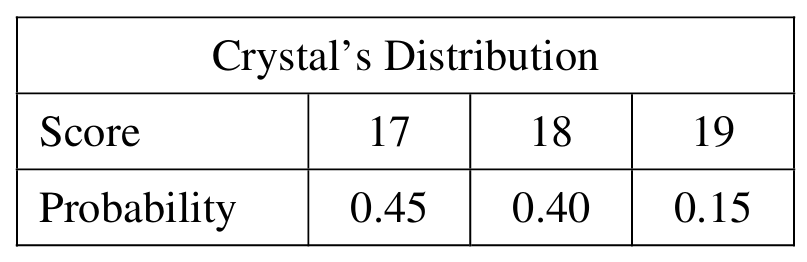

Most-appropriate topic codes (AP Statistics):
• Topic \(2.9\) — Parameters of Random Variables (Part \(\mathrm{a}\))
• Topic \(2.7\) — Independent Events and Unions of Events (Parts \(\mathrm{b}\), \(\mathrm{c}\), \(\mathrm{d}\))
▶️ Answer/Explanation
(a)
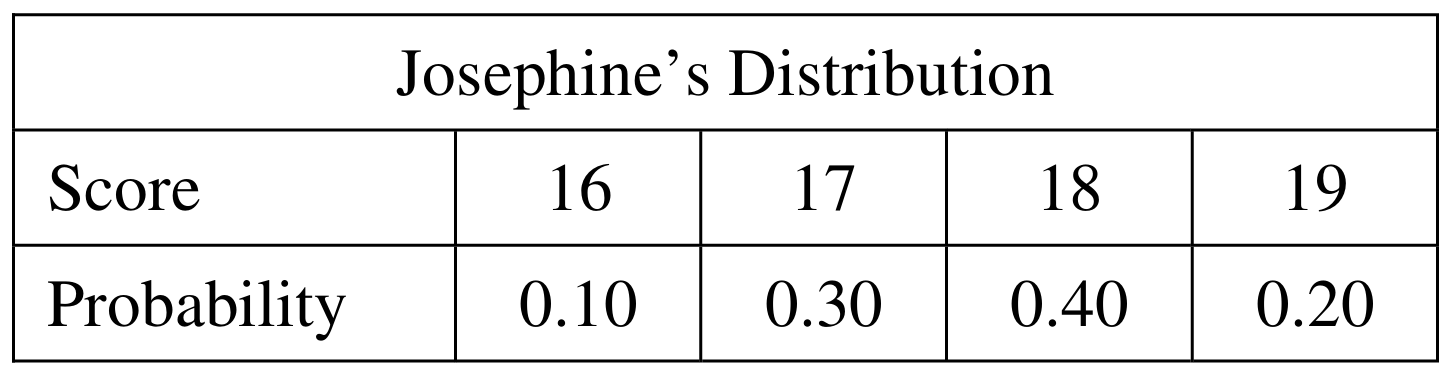
The expected value (mean) of a discrete random variable is \(\mu = \sum x_i \cdot P(x_i)\). We apply this to each player’s distribution.
For Josephine:
\(\mu_J = 16(0.10) + 17(0.30) + 18(0.40) + 19(0.20)\)
\(\mu_J = 1.6 + 5.1 + 7.2 + 3.8 = \boxed{17.7}\)
For Crystal:
\(\mu_C = 17(0.45) + 18(0.40) + 19(0.15)\)
\(\mu_C = 7.65 + 7.20 + 2.85 = \boxed{17.7}\)
Both players have the same expected score of \(17.7\).
(b)
We need all pairs \((J, C)\) such that \(J – C = -1\), i.e., Josephine’s score is exactly 1 less than Crystal’s. Since scores are independent, the probability of each pair is the product of the individual probabilities.
\(J = 16,\ C = 17\): \(\quad P = (0.10)(0.45) = 0.045\)
\(J = 17,\ C = 18\): \(\quad P = (0.30)(0.40) = 0.120\)
\(J = 18,\ C = 19\): \(\quad P = (0.40)(0.15) = 0.060\)
These are the only three combinations that produce a difference of \(-1\).
(c)
Since the three combinations in part (b) are mutually exclusive, we simply add their probabilities:
\(P(J – C = -1) = 0.045 + 0.120 + 0.060\)
\(\boxed{P(J – C = -1) = 0.225}\)
(d)
First, we find the missing probability for a difference of \(-2\). Since all probabilities in the distribution must sum to 1:
\(P(J – C = -2) = 1 – 0.015 – 0.225 – 0.325 – 0.260 – 0.090\)
\(P(J – C = -2) = 1 – 0.915 = \boxed{0.085}\)
The completed distribution table is:

Crystal’s score is higher than Josephine’s when the difference \(J – C < 0\), i.e., when the difference is \(-3\), \(-2\), or \(-1\).
\(P(\text{Crystal} > \text{Josephine}) = P(J – C < 0) = 0.015 + 0.085 + 0.225\)
\(\boxed{P(\text{Crystal} > \text{Josephine}) = 0.325}\)
Question
Most-appropriate topic codes (AP Statistics):
• Topic 1.9 — Comparisons of the Distributions for One Quantitative Variable (Part \(\mathrm{b}\))
• Topic 4.7 — Constructing a Confidence Interval for the Difference Between Two Population Means (Part \(\mathrm{c}\))
• Topic 4.8 — Justifying a Claim Based on a Confidence Interval for the Difference Between Two Population Means (Part \(\mathrm{c}\))
▶️ Answer/Explanation
(a)
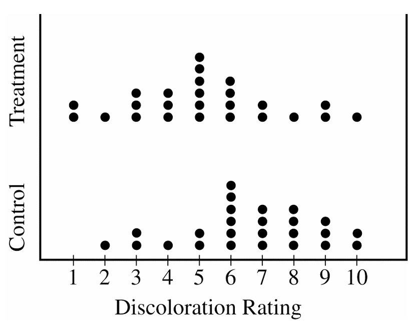
The standard deviation \(s = 2.141\) tells us roughly how far a typical discoloration rating in the control group falls from the group’s mean rating.
In other words, on average, a single strawberry’s discoloration rating in the control group deviates from the mean discoloration rating by about \(2.141\) points.
A larger standard deviation would indicate that the individual ratings are more spread out from the mean, while a smaller value would indicate the ratings are clustered more tightly around the mean.
\(\boxed{s = 2.141 \text{ is the typical distance of each discoloration rating from the mean in the control group.}}\)
(b)
The preservative does appear to have been effective in lowering the amount of discoloration in strawberries.
Looking at the dotplots, the treatment group’s distribution is clearly centered at a lower value than the control group’s distribution — the treatment group’s center is around 5, while the control group’s center is around 7.
Additionally, nearly all the summary statistics (minimum, \(Q_1\), median, and \(Q_3\)) are lower for the treatment group than for the control group, which consistently supports the conclusion that the preservative reduced discoloration.
\(\boxed{\text{The preservative appears effective: treatment ratings are consistently lower than control ratings.}}\)
(c)
We are given a 95% confidence interval for \(\mu_{\text{control}} – \mu_{\text{treatment}}\) as \((0.16,\ 2.72)\).
Since the entire interval lies above zero — meaning zero is not contained within \((0.16,\ 2.72)\) — we have convincing evidence that the two population means are not equal.
We are 95% confident that the population mean discoloration rating for untreated strawberries is between \(0.16\) and \(2.72\) units higher than the population mean rating for treated strawberries, indicating the preservative does make a real difference.
\(\boxed{0 \notin (0.16,\ 2.72) \Rightarrow \text{there is a significant difference in population mean discoloration ratings.}}\)
Question

Most-appropriate topic codes (AP Statistics):
• Topic 4.8 — Justifying a Claim Based on a Confidence Interval for the Difference Between Two Population Means (Part \(\mathrm{b}\))
▶️ Answer/Explanation
(a)
We use a two-sample \(t\)-interval for \(\mu_A – \mu_S\), the difference in mean wait times (Ambulance \(-\) Self).
Conditions:
The 150 patients were randomly selected, so it is reasonable to treat the ambulance and self-transport groups as independent random samples. Both sample sizes are large (\(n_A = 77 > 30\) and \(n_S = 73 > 30\)), so by the Central Limit Theorem the sampling distributions of the sample means are approximately normal.
Mechanics:
Using the conservative degrees of freedom \(df = \min(77-1,\, 73-1) = 72\) and \(t^* = 2.6459\) at the 99% level:
\((\bar{x}_A – \bar{x}_S) \pm t^* \sqrt{\frac{s_A^2}{n_A} + \frac{s_S^2}{n_S}}\)
\((6.04 – 8.30) \pm 2.6459\sqrt{\frac{4.30^2}{77} + \frac{5.16^2}{73}}\)
\(-2.26 \pm 2.6459\sqrt{\frac{18.49}{77} + \frac{26.63}{73}}\)
\(-2.26 \pm 2.6459\sqrt{0.2401 + 0.3648}\)
\(-2.26 \pm 2.6459 \times 0.7778\)
\(-2.26 \pm 2.0577\)
\(\boxed{(-4.318,\ -0.202)}\)
Interpretation: Based on this sample, we are 99% confident that the true difference in population mean wait times (Ambulance \(-\) Self) is between \(-4.318\) minutes and \(-0.202\) minutes. That is, ambulance-transported patients wait, on average, somewhere between about 0.2 and 4.3 minutes less than self-transported patients.
(b)
Yes, the difference in mean wait times is statistically significant at the \(\alpha = 0.01\) level.
Since the value \(0\) is not contained in the 99% confidence interval \((-4.318,\ -0.202)\), we can reject \(H_0: \mu_A – \mu_S = 0\) in favor of \(H_a: \mu_A – \mu_S \neq 0\) at the \(\alpha = 0.01\) significance level.
There is sufficient evidence to conclude that the mean wait time for ambulance-transported patients is significantly different from (specifically, shorter than) the mean wait time for self-transported patients.
\(\boxed{0 \notin (-4.318,\ -0.202) \implies \text{Reject } H_0 \text{ at } \alpha = 0.01}\)
Question

• Connect these two points with a line segment.
• Plot the two means (suburban and urban) for the children who played outside at the two types of day-care centers.
• Connect these two points with a second line segment.
Most-appropriate topic codes (AP Statistics):
• Topic 4.8 — Justifying a Claim Based on a Confidence Interval for the Difference Between Two Population Means (Part a, Part c)
• Topic 5.1 — Graphical Representations Between Two Quantitative Variables (Part b)
▶️ Answer/Explanation
(a)
First check conditions for a two-sample \(t\)-interval: the two groups of urban children were assigned at random and independently to play inside or outside, and dotplots of each group’s data show no strong skew or outliers, so it’s reasonable to treat the underlying populations as approximately normal.

Summary statistics for the urban sample:
\( n_{\text{in}}=9,\quad \bar{x}_{\text{in}}=4.56,\quad s_{\text{in}}=0.846 \)
\( n_{\text{out}}=9,\quad \bar{x}_{\text{out}}=17.56,\quad s_{\text{out}}=4.61 \)
The two-sample \(t\)-confidence interval formula is
\( (\bar{x}_{\text{in}}-\bar{x}_{\text{out}})\pm t^*\sqrt{\dfrac{s_{\text{in}}^2}{n_{\text{in}}}+\dfrac{s_{\text{out}}^2}{n_{\text{out}}}} \)
Using the conservative degrees of freedom \(df=\min(n_{\text{in}}-1,\,n_{\text{out}}-1)=8\), so \(t^*=2.306\):
\( (4.56-17.56)\pm 2.306\sqrt{\dfrac{(0.846)^2}{9}+\dfrac{(4.61)^2}{9}} \)
\( -13.00\pm 2.306(1.564) \)
\( -13.00\pm 3.61 \)
\( \boxed{(-16.60,\ -9.40)\text{ mcg}} \)
Interpretation: we are 95% confident that, for the population of urban day-care children, the mean amount of lead on the dominant hand after an hour of play inside is between 9.40 and 16.60 mcg lower than after an hour of play outside. Since this interval doesn’t contain zero, the difference is meaningful — urban children who play outside pick up noticeably more lead on their hands.
(b)
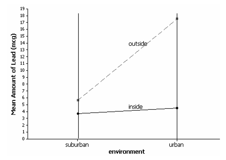
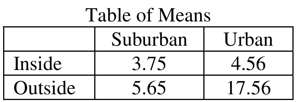
Plot the points \((\text{Suburban},3.75)\) and \((\text{Urban},4.56)\), connect them with a line labeled “inside.” Then plot \((\text{Suburban},5.65)\) and \((\text{Urban},17.56)\), connect them with a line labeled “outside.” The “inside” line should be nearly flat and low on the graph, while the “outside” line should rise sharply from suburban to urban.
\( \boxed{\text{Inside line: nearly flat, low values; Outside line: steep increase from suburban to urban}} \)
(c)
Setting (inside vs. outside): In both suburban and urban environments, children who played outside ended up with more lead on their hands than children who played inside. This is supported by the fact that all four endpoints of the two confidence intervals (inside minus outside) are negative, and the graph shows the “outside” line sitting above the “inside” line everywhere.
Environment (suburban vs. urban): For both inside and outside play, urban children had more lead on their hands on average than suburban children. The graph shows both lines sloping upward from suburban to urban.
Relationship between the two: The effect of going inside versus outside depends heavily on the environment. In the suburban setting, the inside and outside means are fairly close together (3.75 vs. 5.65), but in the urban setting the gap is much larger (4.56 vs. 17.56). In other words, playing outside makes a much bigger difference in lead exposure in the urban environment than in the suburban environment.
\( \boxed{\text{Outside > Inside in both settings; Urban > Suburban in both settings; the inside/outside gap is much larger for urban than suburban}} \)
Question
Most-appropriate topic codes (AP Statistics):
• Topic 4.8 — Justifying a Claim Based on a Confidence Interval for the Difference Between Two Population Means (Part a)
• Topic 4.7 — Constructing a Confidence Interval for the Difference Between Two Population Means (Part b)
▶️ Answer/Explanation
(a)
We use a two-sample \(t\)-interval for the difference in means \((\mu_1 – \mu_2)\), where:
\(\mu_1\) = mean homework time for all sixth-graders at Crest Middle School
\(\mu_2\) = mean homework time for all seventh-graders at Crest Middle School
Assumptions checked: The two samples are independent random samples. The dotplots indicate that it is not unreasonable to assume approximate normality for both groups. So we may proceed.
The general form of the two-sample \(t\)-interval is:
\((\bar{X}_1 – \bar{X}_2) \pm t^* \sqrt{\dfrac{s_1^2}{n_1} + \dfrac{s_2^2}{n_2}}\)
Substituting the values (using sixth-grade as group 1 and seventh-grade as group 2):
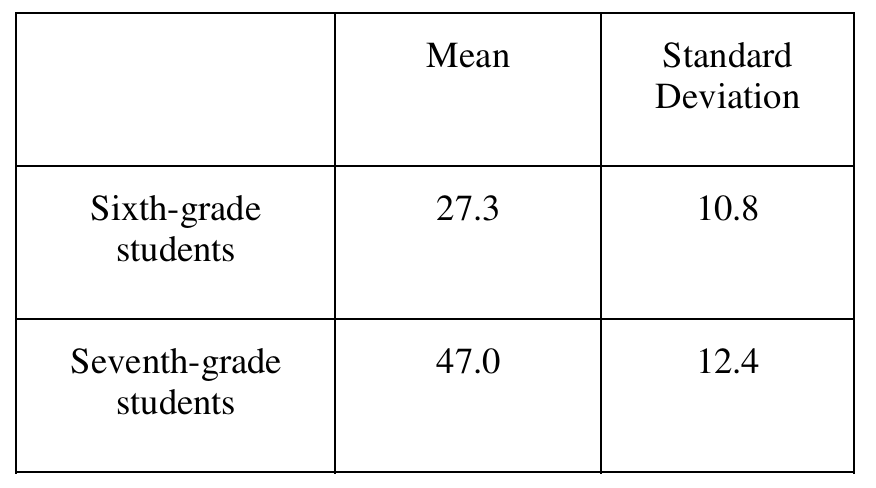
\((27.3 – 47.0) \pm t^* \sqrt{\dfrac{10.8^2}{20} + \dfrac{12.4^2}{20}}\)
\(-19.7 \pm t^* \sqrt{\dfrac{116.64}{20} + \dfrac{153.76}{20}}\)
\(-19.7 \pm t^* \sqrt{5.832 + 7.688} = -19.7 \pm t^* \sqrt{13.52} = -19.7 \pm t^*(3.68)\)
Using \(t^* = 2.026\) based on approximately 37.297 degrees of freedom at a 95% confidence level:
\(-19.7 \pm 2.026 \times 3.68 = -19.7 \pm 7.45\)
\(\boxed{(-27.15,\ -12.25)}\)
Interpretation: Based on these samples, we can be 95% confident that the true difference in mean homework times (sixth-graders minus seventh-graders) for all students at Crest Middle School is between \(-27.15\) minutes and \(-12.25\) minutes. That is, seventh-graders spend, on average, between about 12.25 and 27.15 more minutes per night on homework than sixth-graders.
(b)
No, the assistant principal’s suggestion is not a valid procedure, and it would not produce a better confidence interval. Matching students based on their homework time responses — pairing the highest sixth-grader with the highest seventh-grader, and so on — is inappropriate for two key reasons.
First, valid matched-pairs designs require that pairs be formed before data are collected, based on some variable related to the response (such as prior GPA, study habits, or some pre-existing characteristic), not on the response variable itself. Pairing after the fact on the observed response creates an artificial association between the two independent samples.
Second, because the two samples were drawn independently with no natural connection between any sixth-grader and any seventh-grader, forcing them into pairs based on their ranked responses would artificially inflate the correlation between the paired differences. This would produce a confidence interval that is misleadingly narrow and fails to achieve the stated confidence level, giving a false impression of precision.