AP Statistics 5.5 Least-Squares Regression- Exam Style Questions - MCQs - New Syllabus

Question

Alpaca farmers are aware there is often a linear relationship between the age, in years, of an alpaca and the amount of fleece produced, in ounces per month. The least-squares regression line produced from a random sample is

\[\widehat{\text{Fleece}}=40.8-1.1(\text{Age})\]

Based on the model, what is the expected difference in the amounts of fleece of an alpaca of 5 years and an alpaca of 10 years?

(A) An alpaca of 5 years is expected to produce 1.1 less ounces per month than an alpaca of 10 years.
(B) An alpaca of 5 years and an alpaca of 10 years are both expected to produce 40.8 ounces per month.
(C) An alpaca of 5 years is expected to produce 5.5 less ounces per month than an alpaca of 10 years.
(D) An alpaca of 5 years is expected to produce 5.5 more ounces per month than an alpaca of 10 years.
(E) An alpaca of 5 years is expected to produce 1.1 more ounces per month than an alpaca of 10 years.

▶️ Answer/Explanation

The slope of the regression line is -1.1, which means that for every additional year of age, the predicted fleece production decreases by 1.1 ounces per month.

The age difference between the two alpacas is:

\(10-5=5\text{ years}\)

Therefore, the expected difference in fleece production is:

\((-1.1)(5)=-5.5\text{ ounces}\)

This means the 10-year-old alpaca is expected to produce 5.5 fewer ounces per month than the 5-year-old alpaca. Equivalently, the 5-year-old alpaca is expected to produce 5.5 more ounces per month than the 10-year-old alpaca.

✅ Answer: (D)

Question

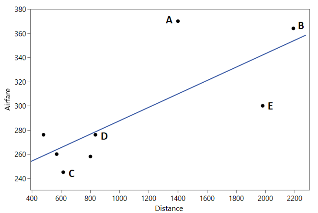
Devon researched the distance of various cities from Atlanta, Georgia compared to the round-trip airfare to each city. Devon’s results are displayed in the scatterplot below.

According to the least squares regression line, which city has the best “value” in airfare based on its distance from Atlanta? A “best value” for this context is defined as having the largest negative residual.

(A) City A
(B) City B
(C) City C
(D) City D
(E) City E

▶️ Answer/Explanation

A residual is calculated as:

\(\text{Residual}=\text{Observed Value}-\text{Predicted Value}\)

A negative residual means the actual airfare is lower than what the regression line predicts. Therefore, the city with the largest negative residual represents the best airfare value for its distance.

Looking at the scatterplot, City E lies well below the regression line and is farther below the line than any of the other labeled cities. City A and City B are above the line (positive residuals), while Cities C and D are only slightly below it.

Therefore, City E has the largest negative residual and thus the best value in airfare based on distance from Atlanta.

✅ Answer: (E)

Question

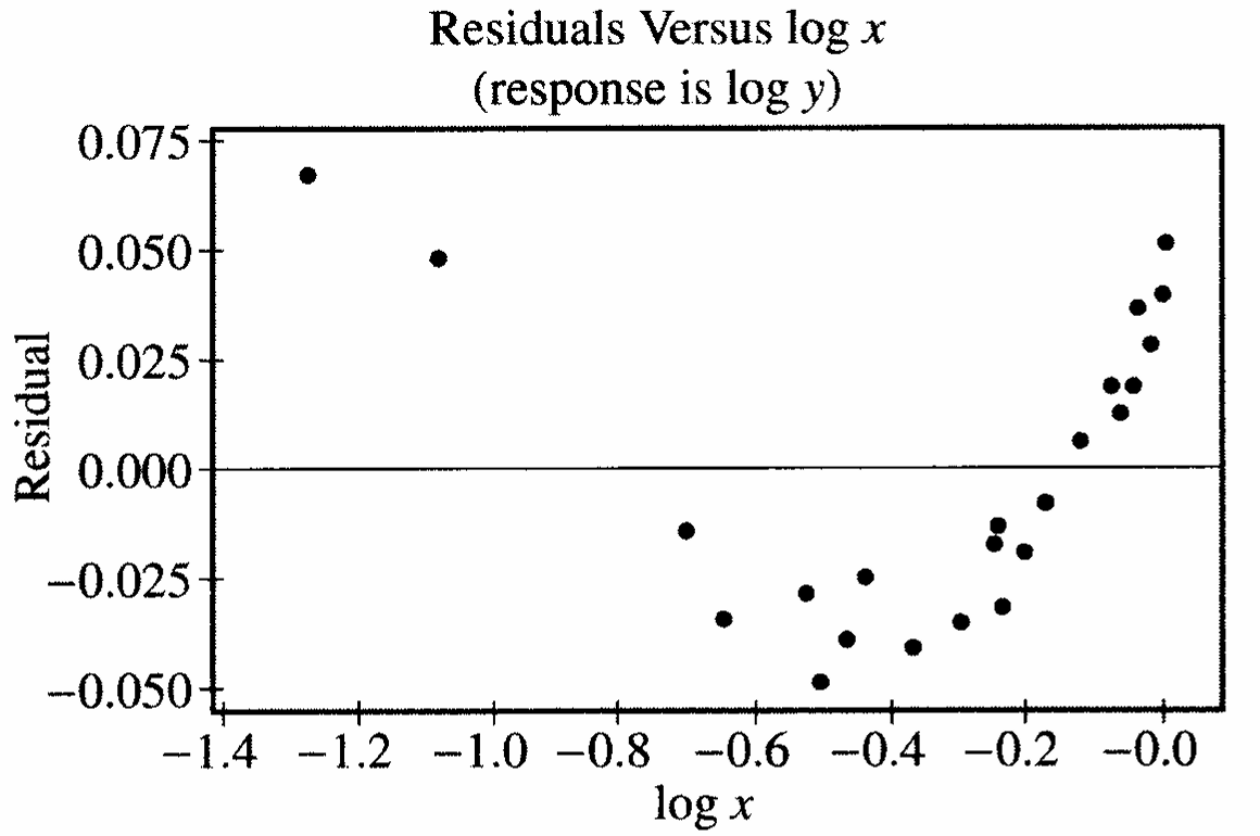
Two variables, \(x\) and \(y\), were measured for a random sample of 25 subjects, and two separate regression models were fit to the data. Least squares estimation of the parameters in Model A yielded the following equation and residual plot.

\[ \widehat{\log y}=0.264+0.230\log x \]

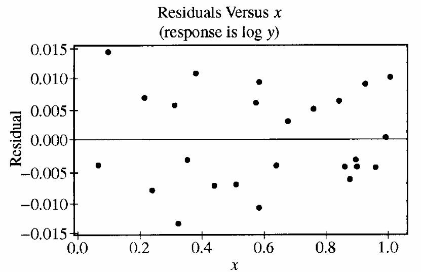
Least squares estimation of the parameters in Model B yielded the following equation and residual plot.

\[ \widehat{\log y}=0.251+0.281x \]

Which of the following conclusions is correct?

(A) Model A is appropriate, since the relationship between \(x\) and \(y\) is linear.

(B) Model B is appropriate, since the relationship between \(x\) and \(y\) is linear.

(C) Model A is appropriate, since the relationship between \(\log x\) and \(\log y\) is linear.

(D) Model A is appropriate, since the relationship between \(\log x\) and \(y\) is linear.

(E) Model B is appropriate, since the relationship between \(x\) and \(\log y\) is linear.

▶️ Answer/Explanation

To determine which model is more appropriate, we examine the residual plots.

For Model A, the residual plot versus \(\log x\) shows a clear curved pattern. The residuals are positive at both ends and negative in the middle, indicating that the linear model does not adequately describe the relationship.

For Model B, the residual plot versus \(x\) shows residuals randomly scattered around zero with no obvious pattern. This suggests that a linear relationship between \(x\) and \(\log y\) is reasonable.

Since the response variable in Model B is \(\log y\), the model assumes a linear relationship between \(x\) and \(\log y\), and the residual plot supports this assumption.

Therefore, Model B is the more appropriate model.

✅ Answer: (E)

AP Statistics 5.5 Least-Squares Regression- Exam Style Questions - MCQs - New Syllabus

Question

Question

Question

Resources

Members

Company