Question 1
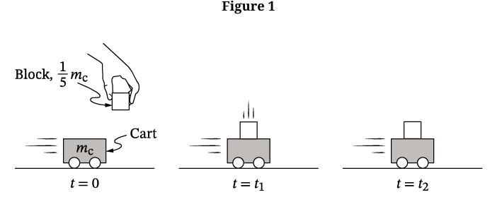
- At time \( t = 0 \), the cart is moving to the right across a horizontal surface with constant speed \( v_c \), and the student releases the block from rest.
- At \( t = t_1 \), the block collides with and sticks to the top of the cart. The block does not slide on the cart.
- At \( t = t_2 \), the block-cart system continues to move to the right with constant speed \( v_f \).
□ Decreases
□ Remains constant
Most-appropriate topic codes (AP Physics 1):
• 3.D.2.1: Conservation of linear momentum — parts A(ii), B
• 5.B.4.1: Kinetic energy — part A(iii)
• 5.B.5.1: Inelastic collisions and energy changes — part A(iii)
• 3.A.2.1: Forces as interactions — part B justification
▶️ Answer/Explanation
(A)(i)
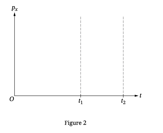
For \( t < t_1 \): Only the cart is moving horizontally with speed \( v_c \), so \( p_x = m_c v_c \).
For \( t > t_1 \): Block and cart stick together; momentum is conserved: \( m_c v_c = \left(m_c + \frac{1}{5}m_c\right) v_f \), so \( p_x = m_c v_c \) remains constant.
✅ Answer: A constant, nonzero, horizontal line from \( t = 0 \) to \( t > t_2 \).

(A)(ii)
Start with conservation of momentum:
\( p_i = p_f \)
\( m_c v_c = \left(m_c + \frac{1}{5}m_c\right) v_f \)
\( m_c v_c = \frac{6}{5}m_c v_f \)
\( v_f = \frac{5}{6} v_c \)
✅ Answer: \( \boxed{v_f = \frac{5}{6} v_c} \).
(A)(iii)
Change in kinetic energy: \( \Delta K = K_f – K_i \)
\( K_i = \frac{1}{2} m_c v_c^2 \)
\( K_f = \frac{1}{2} \left(\frac{6}{5} m_c\right) \left(\frac{5}{6} v_c\right)^2 = \frac{5}{12} m_c v_c^2 \)
\( \Delta K = \frac{5}{12} m_c v_c^2 – \frac{1}{2} m_c v_c^2 = -\frac{1}{12} m_c v_c^2 \)
✅ Answer: \( \boxed{\Delta K = -\frac{1}{12} m_c v_c^2} \).
(B)
The frictional force between block and cart is internal to the block-cart system. No net external force acts on the system in the horizontal direction, so the horizontal momentum remains constant.
✅ Answer: Remains constant.
Justification: The friction is an internal force; only external forces can change the total momentum of a system. Here, the vertical forces are balanced, and no horizontal external force acts.
Question 2
• Shaded bars should start at the dashed line that represents zero energy.
• Represent any energy that is equal to zero with a distinct line on the zero-energy line.
• The relative heights of each shaded bar should reflect the magnitude of the respective
energy consistent with the scale used in Figure 4.
when the block momentarily comes to rest against the compressed spring.
Most-appropriate topic codes (AP Physics 1 Course Framework):
• 4.C.1.1: Calculate the total energy of a system – parts (a), (c)
• 4.C.1.2: Predict changes in the total energy of a system – parts (a), (d)
• 5.B.3.1: Derive an expression for the gravitational potential energy of a system – part (b)
• 5.B.3.2: Derive an expression for the elastic potential energy of a system – part (b)
• 5.B.4.1: Describe and make predictions about the internal energy of systems – part (c)
• 5.B.5.4: Calculate energy changes in processes involving springs – part (b)
• 5.B.5.5: Make calculations of quantities related to energy of a system – part (b)
• 6.B.1.1: Design an experiment for collecting data to determine gravitational potential energy – implied in experimental context
▶️ Answer/Explanation
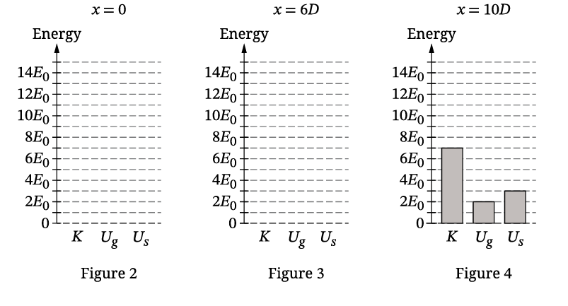
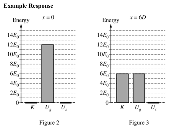
(a) Energy Bar Charts
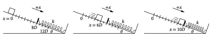
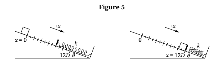
- At \( x = 0 \): Block is at rest (\( K = 0 \)), spring uncompressed (\( U_s = 0 \)), so all energy is gravitational: \( U_g = Mg(12D \sin\theta) = 12E_0 \) (scaled). Only one bar for \( U_g \).
- At \( x = 6D \): Block has descended \( 6D\sin\theta \), so \( U_g = Mg(6D\sin\theta) = 6E_0 \). It has gained kinetic energy: \( K = 6E_0 \). \( U_s = 0 \). Two bars: \( K \) and \( U_g \), each of height \( 6E_0 \).
- Total height of bars in each chart = \( 12E_0 \) (conservation of energy).
Correct charts:
(b) Derivation of \( k \)
Step 1: Write conservation of energy between \( x = 0 \) and \( x = 12D \):
\( U_{g,i} + K_i + U_{s,i} = U_{g,f} + K_f + U_{s,f} \)
Step 2: Substitute known values:
- At \( x = 0 \): \( U_{g,i} = Mg(12D\sin\theta) \), \( K_i = 0 \), \( U_{s,i} = 0 \)
- At \( x = 12D \): \( U_{g,f} = 0 \) (defined), \( K_f = 0 \) (momentarily at rest), \( U_{s,f} = \frac{1}{2}k(\Delta x)^2 \) with \( \Delta x = 4D \)
Step 3: Equation becomes:
\( Mg(12D\sin\theta) = \frac{1}{2}k(4D)^2 \)
Step 4: Solve for \( k \):
\( 12MgD\sin\theta = \frac{1}{2}k(16D^2) \)
\( 12MgD\sin\theta = 8kD^2 \)
\( k = \frac{12Mg\sin\theta}{8D} = \frac{3Mg\sin\theta}{2D} \)
✅ Final expression: \( \boxed{k = \frac{3Mg\sin\theta}{2D}} \)
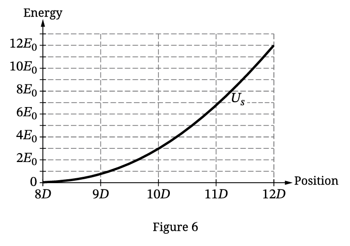
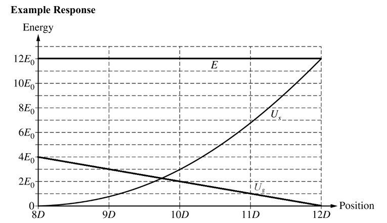
(c) Energy Graphs from \( x = 8D \) to \( 12D \)
- Total mechanical energy \( E \): Constant (no non‑conservative work), horizontal line at \( 12E_0 \).
- Gravitational potential energy \( U_g \): Decreases linearly with \( x \) because \( U_g = Mg(y) \) and \( y = (12D – x)\sin\theta \). At \( x = 8D \), \( U_g = Mg(4D\sin\theta) = 4E_0 \); at \( x = 12D \), \( U_g = 0 \). Straight line from \( (8D, 4E_0) \) to \( (12D, 0) \).
(d) Speed Comparison
Claim: \( v_{9D} > v_{8D} \)
Justification:
From energy conservation: \( K = E – (U_g + U_s) \).
At \( x = 8D \): \( U_g = 4E_0 \), \( U_s = 0 \) ⇒ \( K_{8D} = 12E_0 – 4E_0 = 8E_0 \).
At \( x = 9D \): From the graph, \( U_g \approx 3E_0 \) and \( U_s < E_0 \) (since \( U_s \) curve is below \( E_0 \) at 9D).
Thus \( U_g + U_s < 4E_0 \) ⇒ \( K_{9D} > 8E_0 \).
Since \( K = \frac{1}{2}Mv^2 \) and \( M \) is constant, \( K_{9D} > K_{8D} \) ⇒ \( v_{9D} > v_{8D} \).
✅ Answer: \( \boxed{v_{9D} > v_{8D}} \) with justification referencing energy graph.
Question 3
Most-appropriate topic codes (AP Physics 1):
• 3.F.1.2: Conditions for equilibrium — Part A, Part B
• 5.B.9.1: Graphical analysis and linearization — Part C
• 5.B.10.1: Experimental design and uncertainty — Part A
• 5.B.10.2: Data collection and analysis — Part B, Part C, Part D
▶️ Answer/Explanation
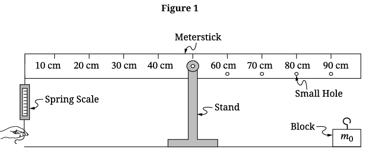
A: Describes a procedure that includes:
- Attaching the block to the meterstick.
- Measuring the force exerted on the left end of the meterstick (spring‑scale reading) while the block is attached and the system is balanced horizontally.
- Indicates a reasonable method to reduce experimental uncertainty (e.g., repeating measurements at one block location, or taking measurements with the block at multiple different hole positions).
B:
- B1: Indicates appropriate quantities that can be plotted so that \( m_0 \) can be determined from the slope (e.g., spring‑scale force \( F \) vs. distance \( d \) from pivot to block, or \( F \) vs. \( d \cdot g \), etc.).
- B2 : Describes how the slope of the graph is related to \( m_0 \).
C:
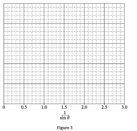
- C1 : Lists a quantity for the vertical axis that yields a linear graph with slope related to \( M \) (e.g., \( F_T \), \( F_T/g \), \( \frac{6F_T}{5g} \), etc.).
- C2 : Correctly labels the vertical axis (with units if appropriate) and uses a linear scale.
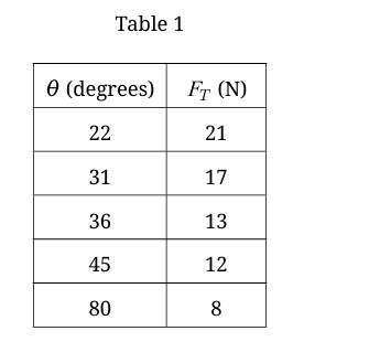
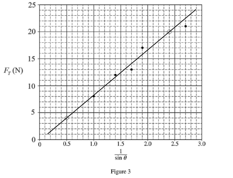
- C3 : Plots data points consistent with the quantities indicated in C(i) or in Table 2.
- C4 : Draws a reasonable straight best‑fit line that approximates the trend of the plotted data.
D:
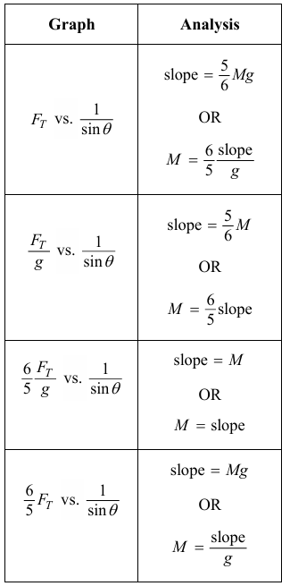
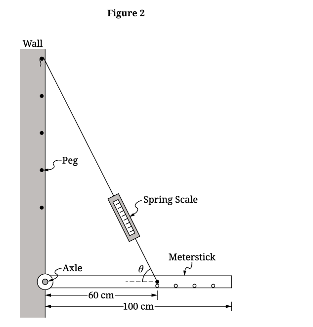
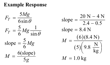
D1 : Correctly relates the slope of the best‑fit line to \( M \) using the given equation \( F_T = \frac{5Mg}{6\sin\theta} \).
- D2 : Calculates a value of \( M \) within the acceptable range (0.90 kg to 1.15 kg).
Key Physics Principles and Methods
1. Torque Equilibrium (Parts A & B)
For the meterstick balanced horizontally about the pivot (stand), the net torque is zero: \[ \tau_{\text{spring scale}} = \tau_{\text{block}}. \] If the spring scale is attached at a fixed distance \( L_s \) from the pivot and the block is at distance \( d \) from the pivot, then \[ F \cdot L_s = m_0 g \cdot d, \] where \( F \) is the spring‑scale reading. Rearranging gives \[ F = \left( \frac{m_0 g}{L_s} \right) d. \] Thus, a graph of \( F \) vs. \( d \) is linear with slope \( \frac{m_0 g}{L_s} \), allowing \( m_0 \) to be determined if \( L_s \) and \( g \) are known.
2. Linearization and Graphical Analysis (Part C)
Given \( F_T = \frac{5Mg}{6\sin\theta} \), rewriting as \[ F_T = \left( \frac{5Mg}{6} \right) \frac{1}{\sin\theta} \] shows that plotting \( F_T \) (vertical) vs. \( \frac{1}{\sin\theta} \) (horizontal) yields a straight line through the origin with slope \( \frac{5Mg}{6} \). Alternative linear forms (e.g., \( \frac{F_T}{g} \) vs. \( \frac{1}{\sin\theta} \)) are also acceptable.
3. Uncertainty Reduction (Part A)
Acceptable methods include: • Taking multiple trials at each block position and averaging. • Using multiple different block positions to obtain several data points for the graph, which reduces the impact of measurement errors.
4. Calculation of \( M \) (Part D)
Using the best‑fit line slope \( k \) from the graph: • If \( F_T \) vs. \( \frac{1}{\sin\theta} \) is plotted, \( k = \frac{5Mg}{6} \), so \( M = \frac{6k}{5g} \). • Using typical values from the data (e.g., slope ≈ 8 N) and \( g = 9.8 \) m/s² gives \( M ≈ 0.98 \) kg, which lies within the acceptable range (0.90–1.15 kg).