▶️ Answer/Explanation
(a)(i)
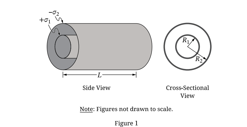
Gauss’s Law: \(\oint \vec{E} \cdot d\vec{A} = \frac{q_{enc}}{\epsilon_{0}}\)
Gaussian surface: Cylinder of radius \(r\) and length \(l\).
\(E(2\pi rl) = \frac{\sigma_{1}(2\pi R_{1}l)}{\epsilon_{0}}\)
\(E = \frac{\sigma_{1}R_{1}}{\epsilon_{0}r}\)
(a)(ii)
Potential Difference: \(|\Delta V| = \left| -\int_{R_{1}}^{R_{2}} E \, dr \right|\)
\(|\Delta V| = \int_{R_{1}}^{R_{2}} \frac{\sigma_{1}R_{1}}{\epsilon_{0}r} \, dr = \frac{\sigma_{1}R_{1}}{\epsilon_{0}} [\ln r]_{R_{1}}^{R_{2}}\)
\(|\Delta V| = \frac{\sigma_{1}R_{1}}{\epsilon_{0}} \ln\left(\frac{R_{2}}{R_{1}}\right)\)
(a)(iii)
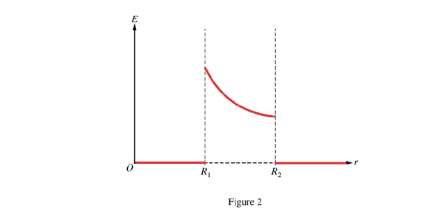
• \(0 < r < R_1\): \(E = 0\) (Inside conductor)
• \(R_1 < r < R_2\): \(E \propto \frac{1}{r}\) (Decreasing, concave up curve)
• \(r > R_2\): \(E = 0\) (Outside neutral capacitor)
(b)
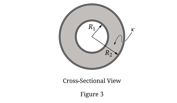
Capacitance definition: \(C = \frac{Q}{|\Delta V|}\) with dielectric \(\kappa\).
Total charge \(Q = \sigma_{1}(2\pi R_{1}L)\).
Potential with dielectric: \(|\Delta V|_{\kappa} = \frac{1}{\kappa} |\Delta V|_{air}\).
\(C = \frac{\sigma_{1} 2\pi R_{1} L}{\frac{1}{\kappa} \frac{\sigma_{1}R_{1}}{\epsilon_{0}} \ln(R_{2}/R_{1})} = \frac{2\pi \kappa \epsilon_{0} L}{\ln(R_{2}/R_{1})}\)
▶️ Answer/Explanation
(a)
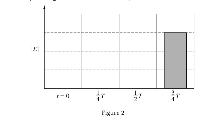
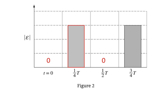
• \(t=0\): Height 0 (Flux is max, Rate of change is 0).
• \(t=\frac{1}{4}T\): Height equal to the bar at \(\frac{3}{4}T\) (Max EMF).
• \(t=\frac{1}{2}T\): Height 0.
(b)
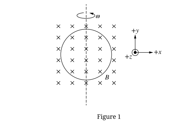
Faraday’s Law: \(\mathcal{E} = -\frac{d\Phi}{dt}\)
\(\mathcal{E} = -\frac{d}{dt}(BA\cos(\omega t)) = -BA(-\omega\sin(\omega t)) = BA\omega\sin(\omega t)\)
Max EMF \(\mathcal{E}_{max} = BA\omega\)
Ohm’s Law: \(I_{max} = \frac{\mathcal{E}_{max}}{R} = \frac{BA\omega}{R}\)
(c)
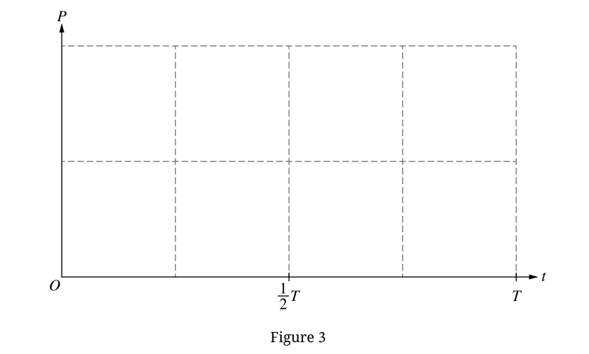
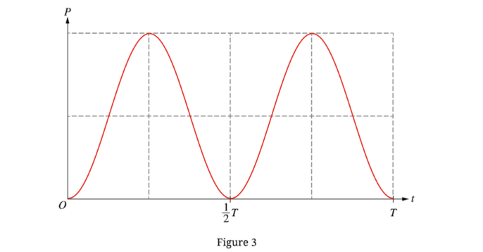
Sketch of \(P\) vs \(t\):
• Starts at \(0\) at \(t=0\).
• Peaks at \(t=\frac{1}{4}T\) and \(t=\frac{3}{4}T\).
• Zero at \(t=\frac{1}{2}T\) and \(t=T\).
• Shape is sinusoidal squared (always positive).
(d)
Consistent.
Relationship: \(P = \frac{\mathcal{E}^2}{R}\).
The power is proportional to the square of the emf. When emf is zero (at \(t=0, T/2\)), power is zero. When emf is maximum (at \(t=T/4, 3T/4\)), power is maximum. This matches the bars in (a) and the peaks in (c).
▶️ Answer/Explanation
(a)
Procedure:
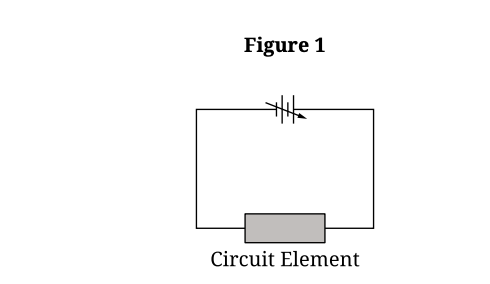
1. Measure the length \(L\) and diameter \(D\) of the cylinder using a ruler or calipers (to calculate Area \(A = \pi(D/2)^2\)).
2. Connect the cylinder in series with an ammeter and power supply, and connect a voltmeter in parallel with the cylinder.
3. Vary the voltage of the power supply to obtain at least 5 different pairs of voltage (\(\Delta V\)) and current (\(I\)) readings.
(b)
Analysis:
• Plot \(\Delta V\) on the vertical axis and \(I\) on the horizontal axis.
• Determine the slope of the best-fit line, which equals the resistance \(R\).
• Calculate resistivity using \(\rho_1 = \frac{R A}{L}\).
(c)
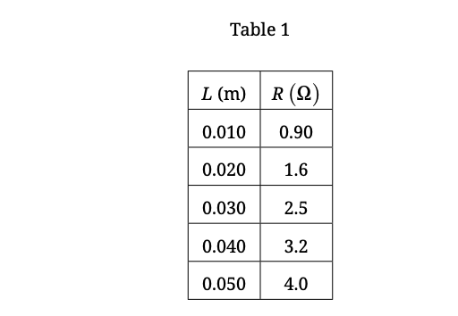
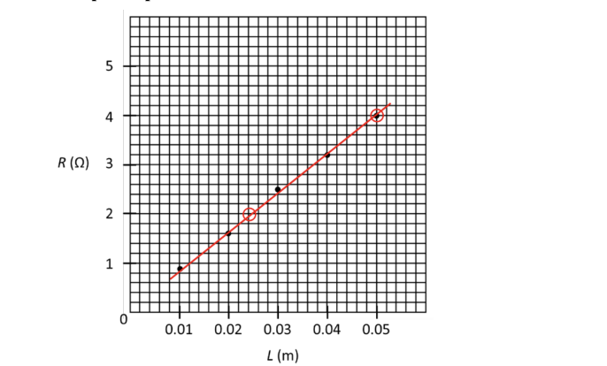
Graph Resistance \(R\) (Vertical) vs. Length \(L\) (Horizontal).
Since \(R = \frac{\rho_2}{A}L\), this plot yields a straight line through the origin.
(d)
Calculation:
• Calculate the slope of the best-fit line from the graph in (c): \(\text{Slope} = \frac{\Delta R}{\Delta L}\).
• Set \(\text{Slope} = \frac{\rho_2}{A}\).
• Solve for \(\rho_2 = \text{Slope} \times A\).
(Example: If Slope \(\approx 77 \, \Omega/m\), then \(\rho_2 \approx 77 \times 5.0 \times 10^{-6} \approx 3.9 \times 10^{-4} \, \Omega \cdot m\)).
▶️ Answer/Explanation
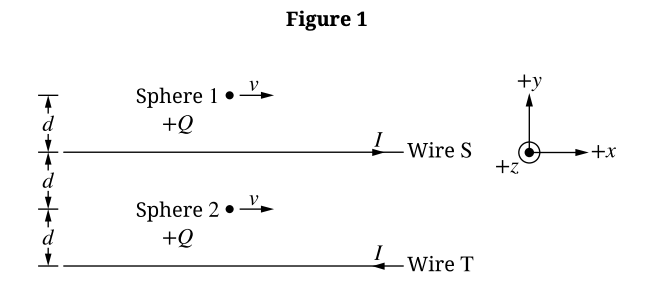
(a)
\(F_{2} > F_{1}\)
At Sphere 2 (between the wires), the magnetic fields from opposite currents point in the same direction and add constructively. At Sphere 1 (outside), the fields point in opposite directions and partially cancel. Since \(F \propto B\), the force is greater at Sphere 2.
(b)
Sphere 2 is distance \(d\) from Wire S and distance \(d\) from Wire T.
Field from a long wire: \(B = \frac{\mu_{0}I}{2\pi r}\).
Since fields add constructively:
\(B_{tot} = B_S + B_T = \frac{\mu_{0}I}{2\pi d} + \frac{\mu_{0}I}{2\pi d} = \frac{2\mu_{0}I}{2\pi d} = \frac{\mu_{0}I}{\pi d}\)
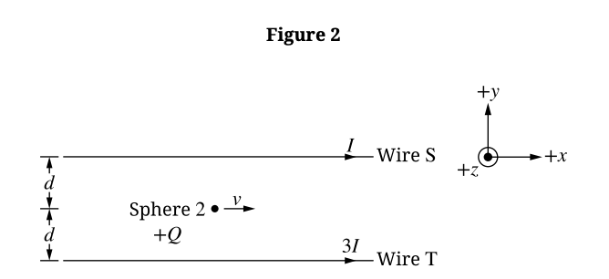
(c)
\(F_{new} = F_{2}\)
In the new scenario, the currents are in the same direction (\(+x\)), so the magnetic fields between the wires now oppose each other (subtract). Wire T has current \(3I\).
\(B_{new} = |B_{T,new} – B_S| = \frac{\mu_{0}(3I)}{2\pi d} – \frac{\mu_{0}I}{2\pi d} = \frac{2\mu_{0}I}{2\pi d} = \frac{\mu_{0}I}{\pi d}\)
The magnitude of the field (and thus the force) remains the same as in part (b).