ap19-frq-statistics

Question 1

The sizes, in square feet, of the $20$ rooms in a student residence hall at a certain university are summarized in the following histogram.

(a) Based on the histogram, write a few sentences describing the distribution of room size in the residence hall.

(b) Summary statistics for the sizes are given in the following table.

Determine whether there are potential outliers in the data. Then use the following grid to sketch a boxplot of room size.

(c) What characteristic of the shape of the distribution of room size is apparent from the histogram but not from the boxplot?

Most-appropriate topic codes (AP Statistics):

• Topic $1.6$ — Describing the Distribution of One Quantitative Variable (Parts $ \mathrm{a} $, $ \mathrm{c} $)
• Topic $1.7$ — Summary Statistics for One Quantitative Variable (Part $ \mathrm{b} $)
• Topic $1.8$ — Graphical Representations of Summary Statistics for One Quantitative Variable (Part $ \mathrm{b} $)

▶️ Answer/Explanation

(a)
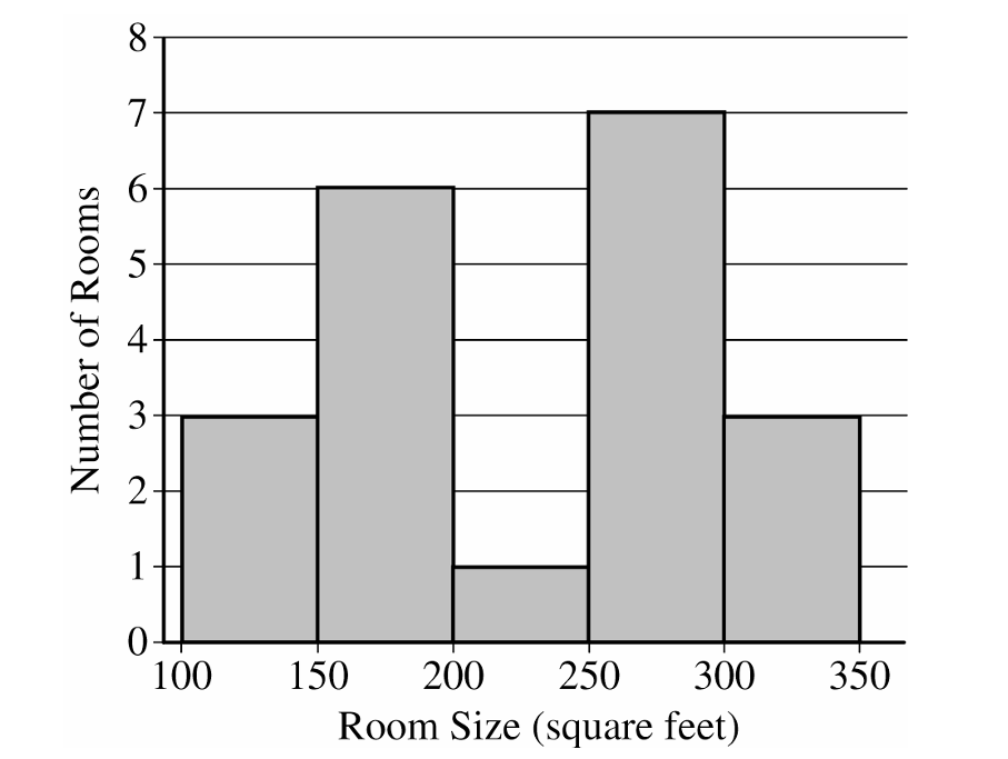
The distribution of the sample of room sizes is bimodal and roughly symmetric.
Most room sizes fall into two clusters: $100$ to $200$ square feet and $250$ to $350$ square feet.
The center of the distribution is between $200$ and $300$ square feet.
The range of the distribution is between $150$ and $250$ square feet.
There are no apparent outliers.

(b)
The interquartile range is:
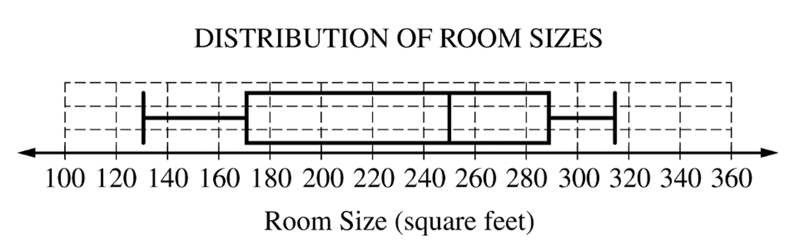
$IQR = Q_3 – Q_1 = 292 – 174 = 118$ square feet.
To find potential outliers, we check the lower and upper fences.
Lower Fence = $Q_1 – 1.5(IQR) = 174 – 1.5(118) = -3$ square feet.
Upper Fence = $Q_3 + 1.5(IQR) = 292 + 1.5(118) = 469$ square feet.
There are no potential outliers because the minimum room size of $134$ square feet does not fall below $-3$, and the maximum room size of $315$ square feet does not exceed $469$.

(c)
The histogram clearly shows the bimodal nature (two peaks or clusters) of the distribution of room sizes.
This bimodal characteristic is not apparent from the boxplot.

Question 2

Researchers are investigating the effectiveness of using a fungus to control the spread of an insect that destroys trees.

The researchers will create four different concentrations of fungus mixtures: $0$ milliliters per liter ($\text{ml/L}$), $1.25\,\text{ml/L}$, $2.5\,\text{ml/L}$, and $3.75\,\text{ml/L}$.

An equal number of the insects will be placed into $20$ individual containers.

The group of insects in each container will be sprayed with one of the four mixtures, and the researchers will record the number of insects that are still alive in each container one week after spraying.

(a) Identify the treatments, experimental units, and response variable of the experiment.

Treatments:

Experimental units:

Response variable:

(b) Does the experiment have a control group? Explain your answer.

(c) Describe how the treatments can be randomly assigned to the experimental units so that each treatment has the same number of units.

Most-appropriate topic codes (AP Statistics):

• Topic $1.10$ — The Investigative Question Revisited and Data Collection (Parts $ \mathrm{a} $, $ \mathrm{b} $)
• Topic $1.13$ — Experimental Design (Part $ \mathrm{c} $)

▶️ Answer/Explanation

(a)
Treatments: The four different concentrations of the fungus spray ($0\,\text{ml/L}$, $1.25\,\text{ml/L}$, $2.5\,\text{ml/L}$, and $3.75\,\text{ml/L}$).
Experimental units: The $20$ individual containers, each containing an equal number of insects.
Response variable: The number of insects that are still alive in each container one week after being sprayed.

(b)
Yes, the experiment definitely has a control group.
The containers sprayed with the $0\,\text{ml/L}$ concentration form the control group because this specific mixture contains absolutely no fungus, serving as a baseline for comparison.

(c)
First, label each of the $20$ containers with a unique integer from $1$ to $20$.
Next, use a random number generator to select $15$ unique integers from $1$ to $20$ without replacement.
Assign the first five containers selected to receive the $0\,\text{ml/L}$ treatment.
Assign the next five containers selected to receive the $1.25\,\text{ml/L}$ treatment, and the next five to receive the $2.5\,\text{ml/L}$ treatment.
Finally, the remaining five containers that were not selected will automatically receive the $3.75\,\text{ml/L}$ treatment.

Question 3

A medical researcher surveyed a large group of men and women about whether they take medicine as prescribed.

The responses were categorized as never, sometimes, or always. The relative frequency of each category is shown in the table.

(a) One person from those surveyed will be selected at random.

i. What is the probability that the person selected will be someone whose response is never and who is a woman?

ii. What is the probability that the person selected will be someone whose response is never or who is a woman?

iii. What is the probability that the person selected will be someone whose response is never given that the person is a woman?

(b) For the people surveyed, are the events of being a person whose response is never and being a woman independent? Justify your answer.

(c) Assume that, in a large population, the probability that a person will always take medicine as prescribed is $0.54$. If $5$ people are selected at random from the population, what is the probability that at least $4$ of the people selected will always take medicine as prescribed? Support your answer.

Most-appropriate topic codes (AP Statistics):

• Topic $2.6$ — Conditional Probability (Part $ \mathrm{a} $)
• Topic $2.7$ — Independent Events and Mutually Exclusive Events (Part $ \mathrm{b} $)
• Topic $2.10$ — The Binomial Distribution (Part $ \mathrm{c} $)

▶️ Answer/Explanation

(a)(i)
From the given two-way table, we can find the joint probability directly by looking at the intersection of the “Women” row and “Never” column.
$P(\text{never and woman}) = 0.0636$

(a)(ii)
To find this probability, we use the general addition rule by adding the marginal probability of “never” to the marginal probability of “woman”, and subtracting their intersection.
$P(\text{never or woman}) = P(\text{never}) + P(\text{woman}) – P(\text{never and woman})$
$P(\text{never or woman}) = 0.1200 + 0.5300 – 0.0636 = 0.5864$

(a)(iii)
For conditional probability, we divide the joint probability of both events occurring by the marginal probability of the given condition (“woman”).
$P(\text{never} \mid \text{woman}) = \dfrac{P(\text{never and woman})}{P(\text{woman})}$
$P(\text{never} \mid \text{woman}) = \dfrac{0.0636}{0.5300} = 0.12$

(b)
We can check for independence by seeing if the conditional probability of an event equals its marginal probability.
Since $P(\text{never} \mid \text{woman}) = 0.12$ and the overall probability $P(\text{never}) = 0.12$, the probabilities are identical.
Yes, this indicates that the event of responding “never” is perfectly independent of the event of being a “woman”.

(c)
This scenario can be modeled using a binomial distribution with $n=5$ trials and a success probability of $p=0.54$.
We need to find the probability of getting at least $4$ successes, which means finding the sum of $P(X=4)$ and $P(X=5)$.
$P(X \ge 4) = \binom{5}{4}(0.54)^4(0.46)^1 + \binom{5}{5}(0.54)^5(0.46)^0$
$P(X \ge 4) \approx 0.19557 + 0.04592 \approx 0.24149$

Question 4

Tumbleweed, commonly found in the western United States, is the dried structure of certain plants that are blown by the wind. Kochia, a type of plant that turns into tumbleweed at the end of the summer, is a problem for farmers because it takes nutrients away from soil that would otherwise go to more beneficial plants. Scientists are concerned that kochia plants are becoming resistant to the most commonly used herbicide, glyphosate.

In $2014$, $19.7$ percent of $61$ randomly selected kochia plants were resistant to glyphosate. In $2017$, $38.5$ percent of $52$ randomly selected kochia plants were resistant to glyphosate.

Do the data provide convincing statistical evidence, at the level of $\alpha=0.05$, that there has been an increase in the proportion of all kochia plants that are resistant to glyphosate?

Most-appropriate topic codes (AP Statistics):

• Topic $3.12$ — Setting Up a Test for the Difference of Two Population Proportions (Entire Question)
• Topic $3.13$ — Carrying Out a Test for the Difference of Two Population Proportions (Entire Question)

▶️ Answer/Explanation

We need to perform a two-sample z-test for a difference in proportions. Let $p_{14}$ and $p_{17}$ be the true proportions of resistant kochia plants in $2014$ and $2017$, respectively.

Our hypotheses are $H_0: p_{17} – p_{14} = 0$ against the alternative $H_a: p_{17} – p_{14} > 0$.

Assuming the samples are independent and random, we calculate the pooled proportion as $\hat{p}_c = \dfrac{61(0.197) + 52(0.385)}{61+52} \approx 0.2835$.

Since the expected counts $61(0.2835)$, $61(1-0.2835)$, $52(0.2835)$, and $52(1-0.2835)$ are all comfortably greater than $10$, the normal condition is satisfied.

Next, we calculate the test statistic: $z = \dfrac{0.385 – 0.197}{\sqrt{0.2835(0.7165)\left(\frac{1}{61} + \frac{1}{52}\right)}} \approx 2.21$.

This gives us a p-value of roughly $0.0135$.

Because the p-value $0.0135$ is less than our significance level $\alpha = 0.05$, we reject $H_0$. There is convincing statistical evidence that the proportion of resistant kochia plants has increased from $2014$ to $2017$.

Question 5

A company that manufactures smartphones developed a new battery that has a longer life span than that of a traditional battery. From the date of purchase of a smartphone, the distribution of the life span of the new battery is approximately normal with mean $30$ months and standard deviation $8$ months. For the price of $\$50$, the company offers a two-year warranty on the new battery for customers who purchase a smartphone. The warranty guarantees that the smartphone will be replaced at no cost to the customer if the battery no longer works within $24$ months from the date of purchase.

(a) In how many months from the date of purchase is it expected that $25$ percent of the batteries will no longer work? Justify your answer.

(b) Suppose one customer who purchases the warranty is selected at random. What is the probability that the customer selected will require a replacement within $24$ months from the date of purchase because the battery no longer works?

(c) The company has a gain of $\$50$ for each customer who purchases a warranty but does not require a replacement. The company has a loss (negative gain) of $\$150$ for each customer who purchases a warranty and does require a replacement. What is the expected value of the gain for the company for each warranty purchased?

Most-appropriate topic codes (AP Statistics):

• Topic $2.8$ — Introduction to Random Variables and Probability Distributions (Part $ \mathrm{c} $)
• Topic $2.9$ — Parameters of Random Variables (Part $ \mathrm{c} $)
• Topic $2.11$ — The Normal Distribution (Parts $ \mathrm{a} $, $ \mathrm{b} $)

▶️ Answer/Explanation

(a)
We need to find the $25\text{th}$ percentile of the normal distribution.
Looking at the standard normal distribution table, the $z$-score that corresponds to a left-tail area of $0.25$ is approximately $-0.6745$.
We can set up the formula for the $z$-score and solve for $x$:
$z = \dfrac{x – \mu}{\sigma}$
$-0.6745 = \dfrac{x – 30}{8}$
$x = 30 + 8(-0.6745) \approx 24.6$
It is expected that $25$ percent of the batteries will no longer work after approximately $24.6$ months.

(b)
We are looking for the probability that the battery lifespan is less than $24$ months.
First, we calculate the $z$-score for $x = 24$:
$z = \dfrac{24 – 30}{8}$
$z = -0.75$
Using the standard normal probability table, the probability $P(Z < -0.75)$ is roughly $0.2266$.
The probability that the customer will require a replacement is $0.2266$.

(c)
Let $X$ represent the company’s financial gain per warranty purchased.
The probability that a replacement is required is $0.2266$, resulting in a loss of $\$150$.
The probability that a replacement is NOT required is $1 – 0.2266 = 0.7734$, resulting in a gain of $\$50$.
The expected value $E(X)$ is the sum of each outcome multiplied by its corresponding probability:
$E(X) = (50)(0.7734) + (-150)(0.2266)$
$E(X) = 38.67 – 33.99$
$E(X) = \$4.68$
The expected gain for the company per warranty purchased is $\$4.68$.

Question 6

Emma is moving to a large city and is investigating typical monthly rental prices of available one-bedroom apartments. She obtained a random sample of rental prices for $50$ one-bedroom apartments taken from a Web site where people voluntarily list available apartments.

(a) Describe the population for which it is appropriate for Emma to generalize the results from her sample.

The distribution of the $50$ rental prices of the available apartments is shown in the following histogram.

(b) Emma wants to estimate the typical rental price of a one-bedroom apartment in the city. Based on the distribution shown, what is a disadvantage of using the mean rather than the median as an estimate of the typical rental price?

(c) Instead of using the sample median as the point estimate for the population median, Emma wants to use an interval estimate. However, computing an interval estimate requires knowing the sampling distribution of the sample median for samples of size $50$. Emma has one point, her sample median, in that sampling distribution.

Using information about rental prices that are available on the Web site, describe how someone could develop a theoretical sampling distribution of the sample median for samples of size $50$.

Because Emma does not have the resources to develop the theoretical sampling distribution, she estimates the sampling distribution of the sample median using a process called bootstrapping. In the bootstrapping process, a computer program performs the following steps.

• Take a random sample, with replacement, of size $50$ from the original sample.
• Calculate and record the median of the sample.
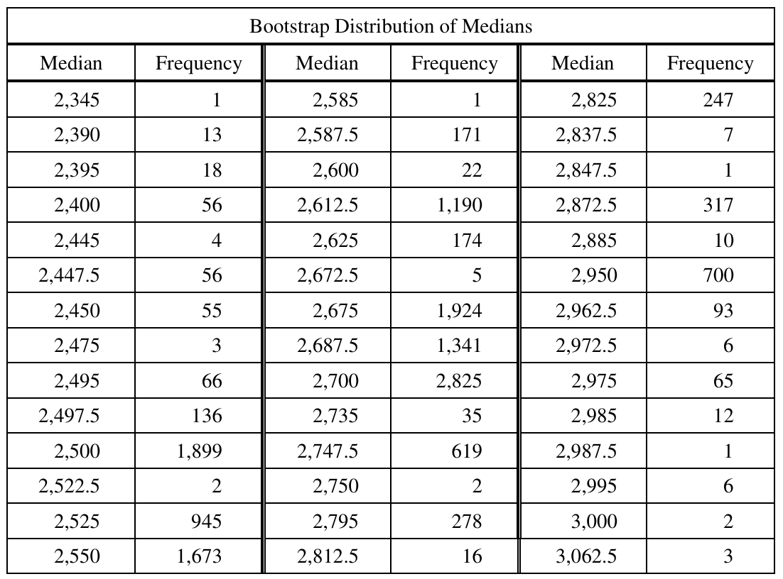
• Repeat the process to obtain a total of $15,000$ medians.

Emma ran the bootstrap process, and the following frequency table is the bootstrap distribution showing her results of generating $15,000$ medians.

The bootstrap distribution provides an approximation of the sampling distribution of the sample median. A confidence interval for the median can be constructed using a percentage of the values in the middle of the bootstrap distribution.

(d) Use the frequency table to find the following.

i. Value of the $5\text{th}$ percentile:

ii. Value of the $95\text{th}$ percentile:

(e) Find the percentage of bootstrap medians in the table that are equal to or between the values found in part (d).

(f) Use your values from parts (d) and (e) to construct and interpret a confidence interval for the median rental price.

Most-appropriate topic codes (AP Statistics):

• Topic $1.11$ — Random Sampling (Part $ \mathrm{a} $)
• Topic $1.12$ — Potential Problems with Sampling (Part $ \mathrm{a} $)
• Topic $1.7$ — Summary Statistics for One Quantitative Variable (Parts $ \mathrm{b} $, $ \mathrm{d} $, $ \mathrm{e} $)
• Topic $2.12$ — Central Limit Theorem and Sampling Distributions for Sample Means (Parts $ \mathrm{c} $, $ \mathrm{f} $)

▶️ Answer/Explanation

(a)
Because a random sample was used, it is appropriate to generalize the results to the population of all rental prices for one-bedroom apartments in the city that are listed on this particular website at the time the sample was taken.

(b)
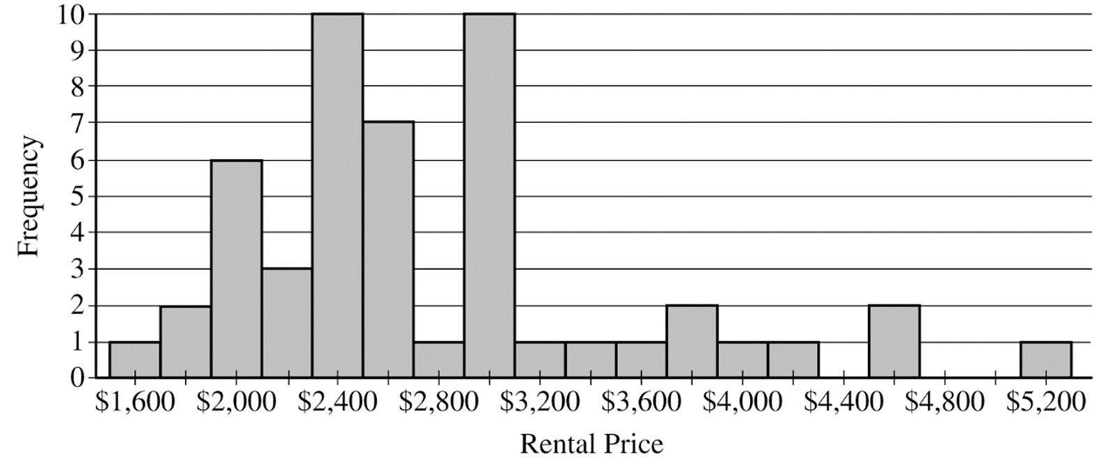
The histogram indicates that the distribution of rental prices is strongly skewed to the right.
Because of this right skewness, the sample mean will be pulled substantially higher by a few very large rental prices.
Consequently, the sample mean would overestimate the typical rental price, whereas the sample median provides a more accurate representation of the center.

(c)
To develop a theoretical sampling distribution, Emma would need to obtain every possible sample of size $50$ from the population of apartments listed on the website.
She would then compute the median rental price for each of these possible samples.
The entire collection of all these computed sample medians forms the theoretical sampling distribution for the sample median.

(d)
i. The $5\text{th}$ percentile corresponds to the $(0.05)(15,000) = 750\text{th}$ value in the ordered data.
By keeping a running cumulative total of the frequencies down the columns, the $750\text{th}$ value first falls in the row for the median of $\$2,500$.
ii. The $95\text{th}$ percentile corresponds to the $(0.95)(15,000) = 14,250\text{th}$ value in the ordered data.
Continuing to add the frequencies, the $14,250\text{th}$ value falls in the row for the median of $\$2,950$.

(e)
We need to sum the frequencies of all bootstrap medians from $\$2,500$ to $\$2,950$ inclusive.
$\text{Sum} = 1,899 + 2 + \dots + 10 + 700 = 14,404$
$\text{Percentage} = \left(\dfrac{14,404}{15,000}\right) \times 100\% \approx 96.03\%$

(f)
Based on our previous parts, an approximate $96\%$ confidence interval for the median is $(\$2,500, \$2,950)$.
Interpretation: We are approximately $96\%$ confident that the true median rental price of all one-bedroom apartments listed on this website for this city is between $\$2,500$ and $\$2,950$.

Question 1

Question 2

Question 3

Question 4

Question 5

Question 6

Resources

Members

Company