Question
The length of stay in a hospital after receiving a particular treatment is of interest to the patient, the hospital, and insurance providers. Of particular interest are unusually short or long lengths of stay. A random sample of 50 patients who received the treatment was selected, and the length of stay, in number of days, was recorded for each patient. The results are summarized in the following table and are shown in the dotplot.

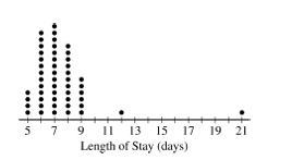
(a) Determine the five-number summary of the distribution of length of stay.
(b) Consider two rules for identifying outliers, method A and method B. Let method A represent the \(1.5 \times \mathrm{IQR}\) rule, and let method \(\mathrm{B}\) represent the 2 standard deviations rule.
(i) Using method A, determine any data points that are potential outliers in the distribution of length of stay. Justify your answer.
(ii) The mean length of stay for the sample is 7.42 days with a standard deviation of 2.37 days. Using method B, determine any data points that are potential outliers in the distribution of length of stay. Justify your answer.
(c) Explain why method A might identify more data points as potential outliers than method B for a distribution that is strongly skewed to the right.
▶️Answer/Explanation
Ans:
mean: 7.42 days
\(\min : 5\) days
max:2ldays
mode:” days is
ronge:16 days
b(i) \(\begin{aligned} & 1 Q R=2 \text { dops } \\ & 2 \cdot 1.5=3 \\ & 7 \pm 3=14,10 \quad \text { of thes } \rightarrow 12,21\end{aligned}\)
(ii)standad deviction \(=2.54\) dets
$
\begin{aligned}
2.37 \cdot 2 & =4.74 \text { dags } \\
& 7.42 \pm 4.74=(2.68,12.16)
\end{aligned}
$
The only data point that method \(B\) describes as an out lat is (d) 21 days.
(c) method \(A\) identified more date points as outlines because the man is skived towers the ing h end the stander deviation is lacier than it wald be in a normally distributed dotyot.
Question
A research center conducted a national survey about teenage behavior. Teens were asked whether they had consumed a soft drink in the past week. The following table shows the counts for three independent random samples from major cities.

(a) Suppose one teen is randomly selected from each city’s sample. A researcher claims that the likelihood of selecting a teen from Baltimore who consumed a soft drink in the past week is less than the likelihood of selecting a teen from either one of the other cities who consumed a soft drink in the past week because Baltimore has the least number of teens who consumed a soft drink. Is the researcher’s claim correct? Explain your answer.
(b) Consider the values in the table. (i) Construct a segmented bar chart of relative frequencies based on the information in the table.

(ii) Which city had the smallest proportion of teens who consumed a soft drink in the previous week? Determine the value of the proportion.
(c) Consider the inference procedure that is appropriate for investigating whether there is a difference among the three cities in the proportion of all teens who consumed a soft drink in the past week.
(i) Identify the appropriate inference procedure.
(ii) Identify the hypotheses of the test.
▶️Answer/Explanation
Ans:
The researcher’s claim is incorrect. Just because the count of Baltimore teens who consumed a soft drink in the past meek doesn’t mean it is leas likely to select a teen from Baltimore who answered yes than the other cities. In reality, the likelihood of a Baltimore teen answering yes is \(\frac{727}{904}=0.804\), which is higher than Detroit \(\left(\frac{1233}{1662}=0.742\right)\) and San Diego \(\left(\frac{1482}{2250}=0,650\right)\). There were differing numbers of teens surveyed in the three cities, so the numbers cannot be compared directly; theymust be proportions first.
(b)

San Diego \(\rightarrow p=\frac{1482}{2280}=0.65\)
(c) The appropriate inference procedure is a \(x^2\)-test for homogeneity.
\(H_s:\) All three cities have the same proportion of teens who consumed a soft drink in the past week.
\(H_a\) : The proportion of teens who had a soft drink in the past week differs among the three cities,
Question
Attendance at games for a certain baseball team is being investigated by the team owner. The following boxplots summarize the attendance, measured as average number of attendees per game, for 47 years of the team’s existence. The boxplots include the 30 years of games played in the old stadium and the 17 years played in the new stadium.
Old Stadium New Stadium

(a) Compare the distributions of average attendance between the old and new stadiums.
The following scatterplot shows average attendance versus year.

(b) Compare the trends in average attendance over time between the old and new stadium.
▶️Answer/Explanation
Ans:
Shape: The distribution of avg attendance at the old stadium is roughly uniform while at the new stadium is skewed to the left.
Center: The median avg attendance at the old stadium is 16,000 attendees while much higher at 25,000 attendees at the new stadium.
Spread: The range of avg attendance at the new stadium (about 12,000 ) is greater than at the old stadium (about 8,000).
Outliers. There is at least one potential outlier of avg attendance at the new stadium at approximately 16,000 attendees.
b) There has been no trend of increasing or decreasing average attendance over time at the old stadium, but average attendance has rapidly increased over time at the new stadium, although the rate of increase is slowing down. The new stadium has seen rapid growth in attendance over the years while the old stadium has seen \(v\) o significant change in trends over time.
c(i) There is a strong positive linear association between the number of games won and average attendance for each year.
(ii) Graph II does rot suggest a change in rate for games in the new stadium compared to the old stadium because there is only a very miner shift io rate between the two clusters of old vs new stadium years and the same regression line could reasonably represent the whole graph.
(d) The number of games won could be a confounding variable in the relationship between average affendance and year or stadium. While the graphs have shown a clear association between year and average attendance (average attendance rapidly increases in 2000 and on) and between stadium and average attendance, (far more people on average attended games at the new stadium than the old stadium), the number of games won in a year is a lurking variable for both of these relationships In the new stadium, the baseball team won way more games per year than they did at the old stadium, but the rate at which average attendance increased with the number of games won didn’t charge when the stadium charged, suggesting the new stadium did n’t cause the increase in average attendance. The average attendance did increase as the years went on, but for most of the years with high attendance (at the new stadium), the team also won more games than before. Therefore, the number of games won per year confounded the relationships between average attendance and year or stadium and explained the average attendance. variation in