Question
Two large corporations, A and B, hire many new college graduates as accountants at entry-level positions. In 2009 the starting salary for an entry-level accountant position was \(\$ 36,000\) a year at both corporations. At each corporation, data were collected from 30 employees who were hired in 2009 as entry-level accountants and were still employed at the corporation five years later. The yearly salaries of the 60 employees in 2014 are summarized in the boxplots below.
(a) Write a few sentences comparing the distributions of the yearly salaries at the two corporations.
(b) Suppose both corporations offered you a job for \(\$ 36,000\) a year as an entry-level accountant.
(i) Based on the boxplots, give one reason why you might choose to accept the job at corporation A.
(ii) Based on the boxplots, give one reason why you might choose to accept the job at corporation B.
▶️Answer/Explanation
Ans:
Corporation \(A\) has a larger range and IQR than Corporation B. Corporation A has two outliers while corporation B has none. Corporation B looks more normal then Cooperation \(A\).
(b) I call choose Corporation A because the maximum salary form the sample of Corporation A was greater then the maximum salary from the sample of corporation B. Therefore, it is possible that after sever l years working there, I too and reach a salary as large as Corporation A’s maximum.
(ii)I could choose corporation B because the minimum salary form the sample for corporation \(B\) is over \(\$ 40,000\) while the minimum from the sample for
Corporation A appears to still be at \$) 36000 which was the starting salary! Therefor, I wald chase corporation \(B\) because if I vent to Compare A I could work there for several years and never get a pay raise in those years.
Question
A shopping mall has three automated teller machines (ATMs). Because the machines receive heavy use, they sometimes stop working and need to be repaired. Let the random variable \(X\) represent the number of ATMs that are working when the mall opens on a randomly selected day. The table shows the probability distribution of \(X\).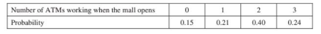
(a) What is the probability that at least one ATM is working when the mall opens?
(b) What is the expected value of the number of ATMs that are working when the mall opens?
(c) What is the probability that all three ATMs are working when the mall opens, given that at least one ATM is working?
(d) Given that at least one ATM is working when the mall opens, would the expected value of the number of ATMs that are working be less than, equal to, or greater than the expected value from part (b) ? Explain.
▶️Answer/Explanation
Ans:
(a)
\(.21+.40+.24 \cdot .85\)
(b) \(\begin{gathered}E(x)=(0 ; 15)+(1 \cdot 21)+(2 \because 40)+(3 \cdot 24) \\ E(x)=1.73\end{gathered}\)
(c)\(\frac{.24}{.85}=.282\)
(d)Equal to because Expected value is calculated by \(\{\) (number of ATM’s) \(\times\) (probabits) so \(\left(0 x_0 15\right)=0\).
Question
A student measured the heights and the arm spans, rounded to the nearest inch, of each person in a random sample of 12 seniors at a high school. A scatterplot of arm span versus height for the 12 seniors is shown.
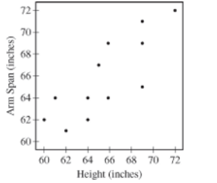
(a) Based on the scatterplot, describe the relationship between arm span and height for the sample of 12 seniors.
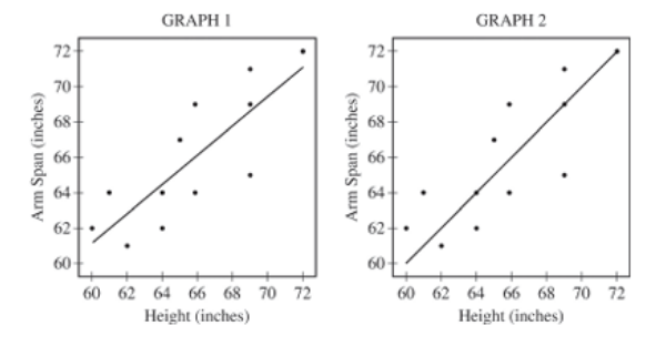
Let \(x\) represent height, in inches, and let \(y\) represent arm span, in inches. Two scatterplots of the same data are shown below. Graph 1 shows the data with the least squares regression line \(\hat{y}=11.74+0.8247 x\), and graph 2 shows the data with the line \(y=x\).
(b) The criteria described in the table below can be used to classify people into one of three body shape categories: square, tall rectangle, or short rectangle.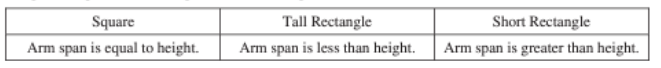
(i) For which graph, 1 or 2, is the line helpful in classifying a student’s body shape as square, tall rectangle, or short rectangle? Explain.
(ii) Complete the table of classifications for the 12 seniors.
(c) Using the best model for prediction, calculate the predicted arm span for a senior with height 61 inches.
▶️Answer/Explanation
Ans:
(a) There is a fairly strong, positive, linear relationship between araspan and height of these 12 seniors.
(b) graph 2. By showing the line \(y=x\) you can determine by the placement of the point whether the arms or heist are longer and/or if the lengths on equal, graph a just displays a best fit line,
\(\begin{array}{ll}\bar{y}=\text { predicted arm span } & \hat{y}=11.74+.8247 x \\ x=\text { height } & \hat{y}=11.74+.8247(61)\end{array}\)
(c) A girl with a 61″ height should here an cromspan of 62.0467 inches according to the least squares regression line.
Question
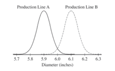
Corn tortillas are made at a large facility that produces 100,000 tortillas per day on each of its two production lines. The distribution of the diameters of the tortillas produced on production line A is approximately normal with mean 5.9 inches, and the distribution of the diameters of the tortillas produced on production line \(\mathrm{B}\) is approximately normal with mean 6.1 inches. The figure below shows the distributions of diameters for the two production lines.
The tortillas produced at the factory are advertised as having a diameter of 6 inches. For the purpose of quality control, a sample of 200 tortillas is selected and the diameters are measured. From the sample of 200 tortillas, the manager of the facility wants to estimate the mean diameter, in inches, of the 200,000 tortillas produced on a given day. Two sampling methods have been proposed.
Method 1: Take a random sample of 200 tortillas from the 200,000 tortillas produced on a given day. Measure the diameter of each selected tortilla.
Method 2: Randomly select one of the two production lines on a given day. Take a random sample of 200 tortillas from the 100,000 tortillas produced by the selected production line. Measure the diameter of each selected tortilla.
(a) Will a sample obtained using Method 2 be representative of the population of all tortillas made that day, with respect to the diameters of the tortillas? Explain why or why not.
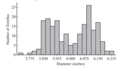
(b) The figure below is a histogram of 200 diameters obtained by using one of the two sampling methods described. Considering the shape of the histogram, explain which method, Method 1 or Method 2, was most likely used to obtain a such a sample.
(c) Which of the two sampling methods, Method 1 or Method 2, will result in less variability in the diameters of the 200 tortillas in the sample on a given day? Explain.
Each day, the distribution of the 200,000 tortillas made that day has mean diameter 6 inches with standard deviation 0.11 inch.
(d) For samples of size 200 taken from one day’s production, describe the sampling distribution of the sample mean diameter for samples that are obtained using Method 1.
(e) Suppose that one of the two sampling methods will be selected and used every day for one year (365 days). The sample mean of the 200 diameters will be recorded each day. Which of the two methods will result in less variability in the distribution of the 365 sample means? Explain.
(f) A government inspector will visit the facility on June 22 to observe the sampling and to determine if the factory is in compliance with the advertised mean diameter of 6 inches. The manager knows that, with both sampling methods, the sample mean is an unbiased estimator of the population mean. However, the manager is unsure which method is more likely to produce a sample mean that is close to 6 inches on the day of sampling. Based on your previous answers, which of the two sampling methods, Method 1 or Method 2, is more likely to produce a sample mean close to 6 inches? Explain.
▶️Answer/Explanation
Ans:
(a)No. Method 2 suffers from selection bias because the sample will not be obtained from the entire population of toxkllas, and the tortillas that are not sampled from will tend to have a different diameter.
Method I
The histogram is bimodal, with a peak \(a+\approx 5.9\) and a peak at z6.1 inches. This means the sample was likely obtained from both production lines, or Method 1.
(c)Method 2.
Because Method 2 obtains the sample from just one production line, the sample will only have one peak, While Method l will nave 2 peaks Thus, Method 2 produces samples with smaller spreads/ standard deviations.
(d)
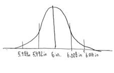
- Because \(n=200 \geq 30\), the central Limit Theorem says that the sampling distribution will be approximately normal.
- The mean of the sampling distribution is equal to the population mean
- the standard deviation is.
$
\sigma_{\bar{x}}=\frac{\sigma}{\sqrt{n}}=\frac{0.11}{\sqrt{200}}=0.00778 \mathrm{in}
$
(e)
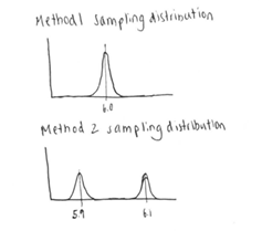
method 1. The sampling distribution tor Method 2 is bimodal, with a peak at \(5.9 \mathrm{in}\) and a peak at \(6.1 \mathrm{in}\), because the samples have means dose to either of these two values. This results in much greater variability in sample means than the unimodal Method sampling distribution.
(f) Methods.
Method 2 is likely to produce a sample mean close to either 5.9 inches or 6.1 inches, depending un the chosen production line, but not close to b.0 inches. Method I selects tortilla as from Both production lines, so the tod’lla diameter tends to average out very close to 6.0 inches.