Home / AP Statistics 1.10 The Normal Distribution Study Notes

AP Statistics 1.10 The Normal Distribution Study Notes

AP Statistics Link- New syllabus

AP Statistics Link Study Notes -As per latest AP Statistics Syllabus.

LEARNING OBJECTIVE

  • The normal distribution can be used to represent some population distributions

Key Concepts:

  • The Normal Distribution Model
  • Determine Proportions and Percentiles from a Normal Distribution

AP Statistics -Concise Summary Notes- All Topics

The Normal Distribution Model

The Normal Distribution Model

The normal distribution is a symmetric, bell-shaped distribution that is fully described by two parameters:

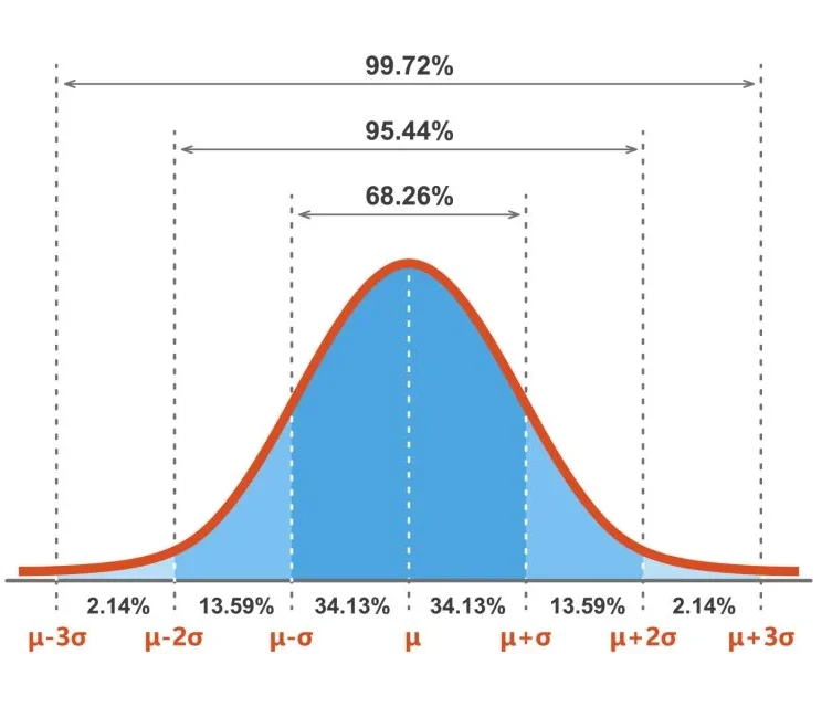
    • \( \mu \) = mean (center of the distribution).
    • \( \sigma \) = standard deviation (controls the spread).

It follows the empirical rule (68–95–99.7 rule):

    • About 68% of data fall within 1 standard deviation of the mean (\( \mu \pm \sigma \)).
    • About 95% within 2 standard deviations (\( \mu \pm 2\sigma \)).
    • About 99.7% within 3 standard deviations (\( \mu \pm 3\sigma \)).

Notation: \( X \sim N(\mu, \sigma) \).

 Comparing a Data Distribution to the Normal Model

Step 1: Shape

  • Check if the distribution is roughly symmetric and bell-shaped.
  • Look for skewness, outliers, or multiple peaks (these indicate non-normality).

Step 2: Center and Spread

  • Compare the sample mean and standard deviation with what would be expected in a normal distribution.
  • Apply the 68–95–99.7 rule to see if data frequencies fit roughly within the expected ranges.

Step 3: Quantitative Tests or Plots

  • Normal probability plot (Q–Q plot): If data are normal, points lie close to a straight diagonal line.
  • Histogram overlay: Compare the histogram of data to a normal curve with the same mean and standard deviation.
  • Boxplot: Check for symmetry and outliers (normal data → symmetric box, no extreme outliers).

 Key Point

In AP Statistics, you must clearly state whether the data are approximately normal or not, and justify based on shape, spread, and adherence to the empirical rule.

Example 

A class of 50 students reports their heights (in cm). The summary statistics are:

  • Mean = 168 cm
  • Standard deviation = 6 cm
  • Minimum = 150 cm
  • Maximum = 185 cm
  • The histogram is roughly symmetric, unimodal, and bell-shaped with no extreme outliers.

 Determine whether the height distribution is approximately normal.

▶️ Answer / Explanation

Step 1: Shape The histogram shows a roughly symmetric and unimodal bell shape. No strong skewness or unusual peaks are observed.

Step 2: Spread (Empirical Rule Check)

  • Mean = 168, SD = 6.
  • \( \mu \pm \sigma \): 162 to 174 → about 34 students (68%) fall here.
  • \( \mu \pm 2\sigma \): 156 to 180 → about 47 students (94%) fall here.
  • \( \mu \pm 3\sigma \): 150 to 186 → all 50 students (100%) fall here.
  • This matches the 68–95–99.7 rule closely.

Step 3: Outliers Minimum = 150, Maximum = 185. Both values are within 3 SDs of the mean, so there are no extreme outliers.

Conclusion: The student heights are approximately normal because the distribution is symmetric, unimodal, follows the empirical rule, and has no outliers.

Determine Proportions and Percentiles from a Normal Distribution

Determine Proportions and Percentiles from a Normal Distribution

Model and z-score

Assume \(X\sim N(\mu,\sigma)\). Convert any value \(x\) to the standard normal using the z-score:

\( z = \dfrac{x – \mu}{\sigma} \).

Finding proportions (areas)

Goal: compute \(P(X<a)\), \(P(X>a)\), or \(P(a<X<b)\).

Methods:

  • Convert endpoints to z-scores: \( z_a = \dfrac{a-\mu}{\sigma} \), \( z_b = \dfrac{b-\mu}{\sigma} \).
  • Use the standard normal CDF \( \Phi(z) \) or a calculator to find areas:
    • \( P(X<a) = \Phi(z_a) \).
    • \( P(X>a) = 1 – \Phi(z_a) \).
    • \( P(a<X<b) = \Phi(z_b) – \Phi(z_a) \).

Calculator commands (TI style):

  • normalcdf(a, b, mu, sigma) gives \(P(a<X<b)\).
  • normalcdf(-1E99, a, mu, sigma) gives \(P(X<a)\).
  • normalcdf(a, 1E99, mu, sigma) gives \(P(X>a)\).

Quick check: the empirical rule says about 68% within \( \mu \pm \sigma \), 95% within \( \mu \pm 2\sigma \), 99.7% within \( \mu \pm 3\sigma \).

Finding percentiles (given area get x)

  • Goal: find the \(p\)th percentile \(x_p\) so that \(P(X \le x_p)=p\).
  • Methods:
    • Find \(z_p\) with \( \Phi(z_p)=p \) (use a table or calculator’s inverse normal).
    • Convert back to the original scale: \( x_p = \mu + z_p \sigma \).
  • Calculator command: use invNorm(p, mu, sigma) to get \(x_p\).

Common z-value shortcuts

  • 50th percentile: \(z=0\).
  • About 16th percentile: \(z\approx -1\).
  • About 84th percentile: \(z\approx +1\).
  • 5th percentile: \(z\approx -1.645\). 95th percentile: \(z\approx +1.645\).
  • 2.5th percentile: \(z\approx -1.96\). 97.5th percentile: \(z\approx +1.96\).
  • 90th percentile: \(z\approx +1.282\).

Example 

 (use \(\mu=168\), \(\sigma=6\))

What proportion of students are taller than 175 cm?

▶️ Answer / Explanation

Compute the z-score: \( z = \dfrac{175 – 168}{6} = \dfrac{7}{6} \approx 1.1667 \).

Lookup \( \Phi(1.1667) \approx 0.8783 \). Then

\( P(X>175) = 1 – \Phi(1.1667) \approx 1 – 0.8783 = 0.1217 \).

Answer: about \(0.1217\) or \(12.17\%\).

Example 

 (use \(\mu=168\), \(\sigma=6\))

 What proportion of students are between 160 cm and 172 cm?

▶️ Answer / Explanation

\( z_{160} = \dfrac{160 – 168}{6} = -\dfrac{8}{6} \approx -1.3333. \)

\( z_{172} = \dfrac{172 – 168}{6} = \dfrac{4}{6} \approx 0.6667. \)

\( \Phi(0.6667) \approx 0.7472,\ \Phi(-1.3333) \approx 0.0909. \)

\( P(160 < X < 172) = 0.7472 – 0.0909 = 0.6563. \)

Answer: about \(0.6563\) or \(65.63\%\).

Example 

 (use \(\mu=168\), \(\sigma=6\))

Find the 90th percentile of student heights.

▶️ Answer / Explanation

Find \(z\) with \( \Phi(z) = 0.90 \). \( z_{0.90} \approx 1.2816 \).

\( x_{0.90} = \mu + z_{0.90} \sigma = 168 + 1.2816(6) \approx 175.69. \)

Answer: about \(175.7\) cm.

Compare Measures of Relative Position in Data Sets

Compare Measures of Relative Position in Data Sets

Percentiles and z-scores are two common measures that allow us to compare where a value lies within a data set, or even across different data sets with different units or scales.

Percentiles

The pth percentile is the value below which $p\%$ of the data fall.

  • Example: The 75th percentile (Q3) means $75\%$ of values are at or below this point.
  • Percentiles describe relative standing within a single data set.

 Z-scores

A z-score measures how many standard deviations a value is from the mean:

\( z = \dfrac{x – \mu}{\sigma} \).

  • A positive z-score means the value is above the mean; negative means below the mean.
  • Z-scores allow comparison across different distributions because they are standardized (unit-free).

Why We Compare

  • Percentiles: Best for describing position within one distribution.
  • Z-scores: Best for comparing across different scales (e.g., test scores, heights, times).
  • Higher z-score → relatively higher standing in the group.

Example

A class has mean test score 70 with standard deviation 8. A student scored 86.

Find the student’s z-score and interpret their relative position.

▶️ Answer / Explanation

\( z = \dfrac{86 – 70}{8} = \dfrac{16}{8} = 2. \)

This student is 2 standard deviations above the mean. They are above about 97.5% of classmates (since \(z=2\) corresponds to the 97.5th percentile).

Example

Alex scores 82 on a math test with mean 75 and standard deviation 5. Bella scores 88 on a science test with mean 80 and standard deviation 6.

 Who performed better relative to their class?

▶️ Answer / Explanation

Compute z-scores:

Alex: \( z = \dfrac{82 – 75}{5} = 1.4 \). Bella: \( z = \dfrac{88 – 80}{6} \approx 1.33 \).

Alex’s z-score is slightly higher, so Alex performed better relative to their group, even though Bella’s raw score is higher.

Example 

A student’s SAT Math score is at the 85th percentile.

 What does this mean about their relative position?

▶️ Answer / Explanation

This means the student scored better than 85% of all test takers. Only 15% scored higher.

Scroll to Top