Describing the Distribution of a Quantitative Variable
When we analyze a quantitative variable, we describe its distribution in terms of its shape, center, spread, and any unusual features. These four elements are often summarized as SOCS (Shape, Outliers, Center, Spread).
Shape of the Distribution
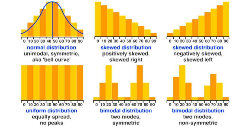
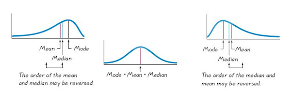
- Symmetric: The left and right halves of the distribution are mirror images. For a symmetric distribution, the mean and median are approximately equal.
- Skewed Right (Positively Skewed): The right tail is longer. A few unusually large values pull the mean above the median.
- Skewed Left (Negatively Skewed): The left tail is longer. A few unusually small values pull the mean below the median.
- Unimodal: The distribution has one clear peak.
- Bimodal: The distribution has two distinct peaks, which may indicate two subgroups in the data.
- Uniform: The data values are spread fairly evenly across the range, with no strong peaks.
Center of the Distribution
- The center represents a “typical” value for the dataset.
- Mean: The arithmetic average. Sensitive to outliers and skewness.
- Median: The middle value when data are ordered. Resistant to outliers and skewness, making it a better choice when data are skewed or contain outliers.
Spread (Variability)
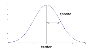
- Spread describes how much the values differ from one another.
- Range: Difference between maximum and minimum values.
- Interquartile Range (IQR): Difference between the third quartile and first quartile, \( IQR = Q_3 – Q_1 \). Resistant to outliers.
- Standard Deviation: Measures average distance from the mean. Sensitive to outliers and skewness.
Unusual Features
- Outliers: Observations that are unusually small or large compared to the rest. They can be detected visually on graphs or using the IQR rule: An observation is considered an outlier if \( x < Q_1 – 1.5 \times IQR \) or \( x > Q_3 + 1.5 \times IQR \).
- Gaps: Empty regions in the data where no observations are recorded. Gaps may suggest separation between groups.
- Clusters: Groups of observations that are bunched together, often separated by gaps.
- Multiple Peaks: Two or more prominent high points in the distribution indicate subgroups or distinct patterns in the data.
Important Note
Descriptive statistics only summarize the dataset at hand. They do not allow us to make conclusions about a larger population. However, they provide patterns and clues that can guide future inferential analysis.
Example :
The math test scores of 20 students are:
72, 75, 76, 78, 79, 80, 81, 82, 83, 84, 85, 85, 86, 87, 88, 89, 90, 91, 92, 93
Describe the distribution of the test scores using SOCS (Shape, Outliers, Center, Spread).
▶️ Answer/Explanation
Shape: The distribution is roughly symmetric and unimodal, centered around the mid-80s.
Outliers: No unusually high or low values are present.
Center: The mean and median are both about 85, showing balance.
Spread: The scores range from 72 to 93 (range = 21). The standard deviation is moderate.
Final Description: The distribution of test scores is symmetric, unimodal, centered at about 85, with no outliers and moderate spread.
Example :
The daily number of minutes 15 people spend on a fitness app are:
2, 4, 5, 6, 7, 8, 10, 12, 15, 18, 20, 22, 25, 60, 120
Describe the distribution of app usage times using SOCS.
▶️ Answer/Explanation
Shape: The distribution is skewed to the right because of a few very large values.
Outliers: The values 60 and 120 are clear outliers.
Center: The median is about 12 minutes, while the mean is higher (≈21) due to outliers.
Spread: The range is large (2 to 120). The IQR is much smaller (≈6 to 22), showing most people use the app moderately.
Final Description: The distribution of app usage is right-skewed with two outliers, a median of 12, and a wide overall spread.
Example :
The weights (in kg) of 22 packages are:
2, 3, 3, 4, 5, 6, 7, 7, 8, 8, 9, 9, 20, 21, 22, 22, 23, 24, 25, 26, 27, 28
Describe the distribution of package weights using SOCS.
▶️ Answer/Explanation
Shape: The distribution is bimodal with two clusters: one around 3–9 kg and another around 20–28 kg. A clear gap exists between 9 and 20.
Outliers: No single value is far from its cluster, so there are no strong outliers.
Center: The median is about 13, but this is misleading because of two distinct groups. Each cluster has its own center (≈6 and ≈23).
Spread: The range is 26 (2 to 28). High variability exists because of the two separated groups.
Final Description: The distribution of package weights is bimodal with two clusters, separated by a gap, no strong outliers, and a wide overall spread.