
1.7.A Calculate Measures of Center and Position for Quantitative Data
When analyzing quantitative data, statisticians often want to identify a value that represents the center of the distribution.
Measures of center describe the typical value in a data set.
Measures of position describe where a particular value is located relative to the rest of the data.
Some of the most important measures of center and position include:
- Mean
- Median
- Minimum and Maximum
- Quartiles
- Percentiles
These measures help summarize large data sets and provide information about the distribution of the data.
1.7.A.1 Measures of Center: Mean and Median
A measure of center is a numerical value that represents the middle or typical value of a distribution.
The two most commonly used measures of center are: 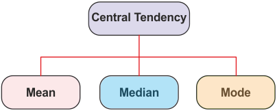
- Mean
- Median
Mean
The mean is commonly called the average.
It uses every value in the data set and is calculated by adding all values and dividing by the number of observations.
Median
The median is the middle value in an ordered data set.
- Half of the observations lie below the median and half lie above it.
- Unlike the mean, the median is not strongly affected by unusually large or unusually small values.
| Measure | Description |
|---|---|
| Mean | Arithmetic average of all values |
| Median | Middle value in ordered data |
The choice between mean and median often depends on the shape of the distribution.
- For symmetric distributions, the mean and median are usually similar.
- For skewed distributions, the median is often preferred because it is resistant to outliers.
Example
The following data represent the number of hours students studied for an exam:
\( \mathrm{2,\ 4,\ 5,\ 6,\ 8} \)
Identify the two measures of center that could be used to describe this data set.
▶️ Answer / Explanation
The two commonly used measures of center are:
- Mean
- Median
Both measures describe the typical study time for the students.
The mean uses all values in the calculation, while the median identifies the middle value of the ordered data set.
1.7.A.2 Mean
The mean is the arithmetic average of a set of quantitative data.
It is calculated by adding all observations and dividing by the total number of observations.
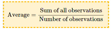
For a sample, the mean is represented by:
$\bar{x}=\frac{\sum x_i}{n}$
where:
- \( \mathrm{x_i} \) represents an individual data value
- \( \mathrm{n} \) represents the sample size
- \( \mathrm{\bar{x}} \) represents the sample mean
Steps for calculating the mean:
- Add all data values.
- Count the number of observations.
- Divide the sum by the number of observations.
The mean uses every value in the data set.
Because of this, extremely large or small values can greatly influence the mean.
Example
Calculate the mean of the following data set:
\( \mathrm{4,\ 6,\ 8,\ 10,\ 12} \)
▶️ Answer / Explanation
Step 1: Find the sum of the values.
\( \mathrm{4+6+8+10+12=40} \)
Step 2: Count the number of observations.
\( \mathrm{n=5} \)
Step 3: Apply the mean formula.
\( \mathrm{\bar{x}=\dfrac{40}{5}=8} \)
Therefore, the mean is:
\( \mathrm{8} \)
1.7.A.3 Median
The median is the middle value in an ordered data set.
- Before finding the median, the data must be arranged from smallest to largest.
- The method used depends on whether the number of observations is odd or even.
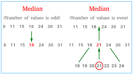
Formula / Method for Finding the Median
Step 1: Arrange the data from smallest to largest.
Step 2: Determine whether the number of observations (\(n\)) is odd or even.
If \(n\) is odd:
$ \text{Median}=\text{Middle Value} $
$\text{Position of Median}=\frac{n+1}{2}$
This gives the location of the middle value in the ordered data set.
If \(n\) is even
$ \text{Median}=\frac{\text{Two Middle Values}}{2} $
Equivalently,
$ \text{Median}=\frac{x_{\frac{n}{2}}+x_{\frac{n}{2}+1}}{2} $
where the data are arranged in ascending order.
| Number of Values | How to Find the Median |
|---|---|
| Odd | Choose the middle value |
| Even | Average the two middle values |
The median is resistant to outliers because it depends only on the position of values rather than their magnitudes.
Example
Find the median of the following data set:
\( \mathrm{3,\ 5,\ 7,\ 9,\ 11,\ 13,\ 15} \)
▶️ Answer / Explanation
Step 1: Verify that the data are ordered.
\( \mathrm{3,\ 5,\ 7,\ 9,\ 11,\ 13,\ 15} \)
Step 2: Count the observations.
\( \mathrm{n=7} \)
Since there is an odd number of values, the median is the middle value.
The fourth value is:
\( \mathrm{9} \)
Therefore, the median is:
\( \mathrm{9} \)
1.7.A.4 Minimum and Maximum Values
In an ordered data set, the smallest value is called the minimum value and the largest value is called the maximum value.
These values identify the endpoints of the distribution.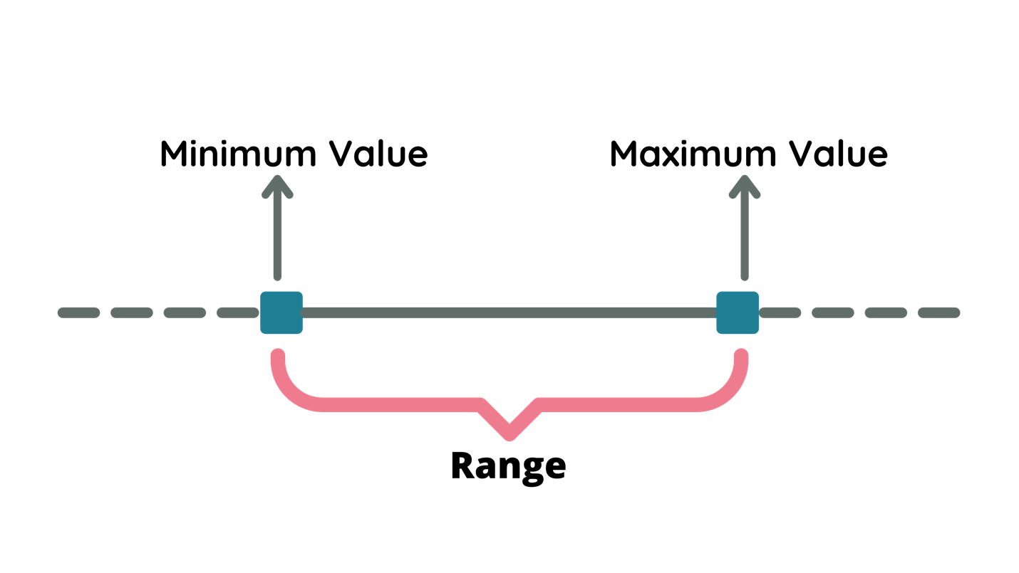
The minimum and maximum values help describe:
- The spread of the data
- The overall range of values
- The boundaries of the distribution
Definitions
- Minimum: Smallest value in the ordered data set
- Maximum: Largest value in the ordered data set
Formula
\( \text{Range}=\text{Maximum}-\text{Minimum} \)
Although range is studied later as a measure of variability, it is calculated directly from the minimum and maximum values.
| Measure | Meaning |
|---|---|
| Minimum | Smallest value in the data set |
| Maximum | Largest value in the data set |
Example
The following test scores were recorded:
\( \mathrm{58,\ 64,\ 70,\ 72,\ 75,\ 81,\ 89} \)
Identify the minimum value and maximum value.
▶️ Answer / Explanation
The smallest value is:
\( \mathrm{58} \)
Therefore, the minimum value is:
\( \mathrm{58} \)
The largest value is:
\( \mathrm{89} \)
Therefore, the maximum value is:
\( \mathrm{89} \)
1.7.A.5 Quartiles (Q1, Q2, Q3)
Quartiles divide an ordered data set into four approximately equal parts.
The three quartiles are:
- \( \mathrm{Q_1} \) (First Quartile)
- \( \mathrm{Q_2} \) (Second Quartile or Median)
- \( \mathrm{Q_3} \) (Third Quartile)
Quartiles help describe the position of data values within a distribution.
First Quartile (Q1)
\( \mathrm{Q_1} \) is the median of the lower half of the ordered data.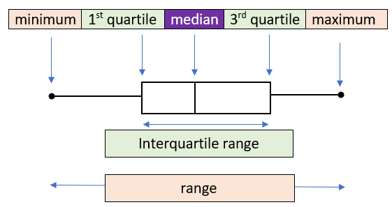
Approximately: \( \mathrm{25\%} \)
of the observations are less than or equal to \( \mathrm{Q_1} \).
Second Quartile (Q2)
\( \mathrm{Q_2} \) is the median of the entire data set.
Approximately: \( \mathrm{50\%} \)
of the observations are less than or equal to \( \mathrm{Q_2} \).
Third Quartile (Q3)
\( \mathrm{Q_3} \) is the median of the upper half of the ordered data.
Approximately: \( \mathrm{75\%} \)
of the observations are less than or equal to \( \mathrm{Q_3} \).
Method for Finding Quartiles
- Order the data from smallest to largest.
- Find the median (\(Q_2\)).
- Find the median of the lower half (\(Q_1\)).
- Find the median of the upper half (\(Q_3\)).
\( \mathrm{Q_1} \) and \( \mathrm{Q_3} \) form the boundaries of the middle 50% of the data.
| Quartile | Percent of Data Below It |
|---|---|
| \( \mathrm{Q_1} \) | 25% |
| \( \mathrm{Q_2} \) | 50% |
| \( \mathrm{Q_3} \) | 75% |
Example
Find \( \mathrm{Q_1} \), \( \mathrm{Q_2} \), and \( \mathrm{Q_3} \) for the following data set:
\( \mathrm{2,\ 4,\ 6,\ 8,\ 10,\ 12,\ 14,\ 16,\ 18} \)
▶️ Answer / Explanation
Step 1: Find the median.
\( \mathrm{Q_2=10} \)
Lower half:
\( \mathrm{2,\ 4,\ 6,\ 8} \)
Upper half:
\( \mathrm{12,\ 14,\ 16,\ 18} \)
Step 2: Find \( \mathrm{Q_1} \).
\( \mathrm{Q_1=\dfrac{4+6}{2}=5} \)
Step 3: Find \( \mathrm{Q_3} \).
\( \mathrm{Q_3=\dfrac{14+16}{2}=15} \)
Therefore:
\( \mathrm{Q_1=5,\ Q_2=10,\ Q_3=15} \)
1.7.A.6 Percentiles
A percentile indicates the position of a value within an ordered data set.
The pth percentile is the value that has approximately: \( \mathrm{p\%} \) of the observations less than or equal to it.
Percentiles help determine how a particular observation compares with the rest of the data.
Definition
\( \text{pth Percentile} = \text{Value with } p\% \text{ of observations at or below it} \)
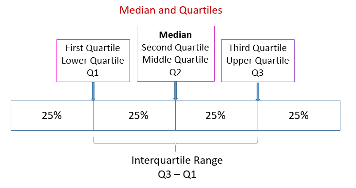
Common percentiles include:
| Percentile | Equivalent Quartile |
|---|---|
| 25th Percentile | \( \mathrm{Q_1} \) |
| 50th Percentile | \( \mathrm{Q_2} \) (Median) |
| 75th Percentile | \( \mathrm{Q_3} \) |
Percentiles are commonly used in:
- Standardized testing
- Growth charts
- Ranking systems
- Educational assessments
Example
A student scored at the 90th percentile on a standardized exam.
Interpret this percentile in context.
▶️ Answer / Explanation
Being at the 90th percentile means the student’s score was greater than or equal to approximately:
\( \mathrm{90\%} \)
of all scores in the distribution.
Only about:
\( \mathrm{10\%} \)
of students scored higher.
Therefore, the student performed better than most students who took the exam.
1.7.B Calculate Measures of Variability for Quantitative Data
While measures of center describe the typical value of a distribution, measures of variability describe how spread out the data values are.
Two data sets may have the same center but very different amounts of variability.
Measures of variability help statisticians understand:
- How much the data vary
- How closely values cluster around the center
- Whether the distribution is tightly packed or widely spread
The three most commonly used measures of variability are:
- Range
- Interquartile Range (IQR)
- Standard Deviation
1.7.B.1 Measures of Variability
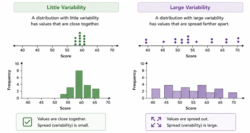
Measures of variability describe the spread of a quantitative distribution.
- A distribution with little variability has values that are close together.
- A distribution with large variability has values that are spread farther apart.
| Measure | Description |
|---|---|
| Range | Distance from minimum to maximum |
| Interquartile Range (IQR) | Spread of the middle 50% of data |
| Standard Deviation | Typical distance from the mean |
Different measures of variability are useful in different situations.
- Range uses only the smallest and largest values.
- IQR focuses on the middle 50% of the data.
- Standard deviation uses every observation.
Example
Two classes have the same mean test score of: \( \mathrm{80} \)
Class A scores range from: \( \mathrm{78} \) to: \( \mathrm{82} \)
Class B scores range from: \( \mathrm{50} \) to: \( \mathrm{100} \)
Which class has greater variability?
▶️ Answer / Explanation
Class B has greater variability.
Although both classes have the same mean, Class B’s scores are spread over a much wider interval.
This indicates that the data values vary more from one another.
1.7.B.2 Range
The range measures the total spread of a data set.
It is calculated using only the minimum value and maximum value.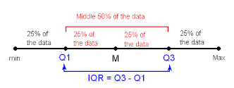
Formula
\( \text{Range}=\text{Maximum}-\text{Minimum} \)
where:
- Maximum = largest value in the data set
- Minimum = smallest value in the data set
A larger range indicates greater variability.
A smaller range indicates less variability.
One limitation of range is that it depends only on two values and can be greatly affected by outliers.
| Minimum | Maximum | Range |
|---|---|---|
| 12 | 32 | 20 |
Example
The following data represent the number of books read by students:
\( \mathrm{3,\ 5,\ 8,\ 10,\ 12,\ 15} \)
Calculate the range.
▶️ Answer / Explanation
Step 1: Identify the minimum and maximum values.
Minimum:
\( \mathrm{3} \)
Maximum:
\( \mathrm{15} \)
Step 2: Apply the formula.
\( \text{Range}=15-3 \)
\( \text{Range}=12 \)
Therefore, the range is:
\( \mathrm{12} \)
1.7.B.3 Interquartile Range (IQR)
The Interquartile Range (IQR) measures the spread of the middle 50% of a data set.
- Because it uses quartiles rather than extreme values, the IQR is resistant to outliers.
- The IQR is the distance between the third quartile and the first quartile.
Formula
\( \mathrm{IQR}=Q_3-Q_1 \)
where:
- \( \mathrm{Q_1} \) = First Quartile (25th percentile)
- \( \mathrm{Q_3} \) = Third Quartile (75th percentile)
The IQR contains the middle: \( \mathrm{50\%} \) of all observations.
A larger IQR indicates greater variability among the middle half of the data.
A smaller IQR indicates that the middle half of the data is more concentrated.
| Measure | Formula |
|---|---|
| Interquartile Range | \( \mathrm{IQR=Q_3-Q_1} \) |
Example
A data set has: \( \mathrm{Q_1=18} \) and \( \mathrm{Q_3=34} \)
Calculate the interquartile range.
▶️ Answer / Explanation
Step 1: Apply the IQR formula.
\( \mathrm{IQR}=Q_3-Q_1 \)
\( \mathrm{IQR}=34-18 \)
\( \mathrm{IQR}=16 \)
Therefore, the interquartile range is:
\( \mathrm{16} \)
This means the middle 50% of the observations span:
\( \mathrm{16} \)
units.
1.7.B.4 Standard Deviation
The standard deviation measures the typical distance that data values lie from the mean of a distribution.
It describes how spread out the data are around the center.
- A small standard deviation indicates that most values are close to the mean.
- A large standard deviation indicates that values are spread farther from the mean.
- Unlike the range, which uses only two observations, standard deviation uses every value in the data set.
For a sample, the standard deviation is represented by: \( \mathrm{s} \)
Formula for Sample Standard Deviation
\( s=\sqrt{\frac{1}{n-1}\sum_{i=1}^{n}(x_i-\bar{x})^2} \)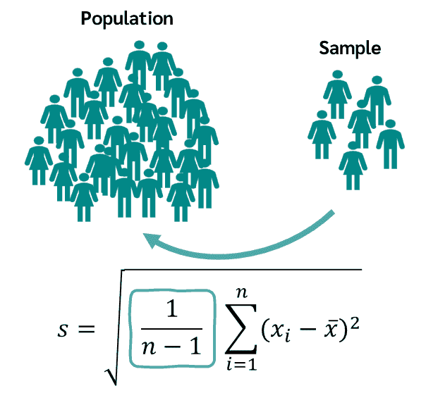
where:
- \( \mathrm{s} \) = sample standard deviation
- \( \mathrm{x_i} \) = individual data value
- \( \mathrm{\bar{x}} \) = sample mean
- \( \mathrm{n} \) = sample size
- \( \mathrm{(x_i-\bar{x})} \) = deviation from the mean
The standard deviation is calculated by:
- Finding the mean.
- Subtracting the mean from each observation.
- Squaring each deviation.
- Adding the squared deviations.
- Dividing by \( \mathrm{n-1} \).
- Taking the square root.
Because this process is lengthy, standard deviation is often calculated using technology in AP Statistics.
Sample Variance
The square of the sample standard deviation is called the sample variance.
It is represented by: \( \mathrm{s^2} \)
Formula for Sample Variance
\( s^2=\frac{1}{n-1}\sum_{i=1}^{n}(x_i-\bar{x})^2 \)
Variance and standard deviation contain the same information about variability, but standard deviation is usually easier to interpret because it is measured in the same units as the original data.
| Measure | Meaning |
|---|---|
| \( \mathrm{s} \) | Sample Standard Deviation |
| \( \mathrm{s^2} \) | Sample Variance |
Interpreting Standard Deviation
- Small standard deviation → data values are close to the mean.
- Large standard deviation → data values are spread farther from the mean.
For example:
- A class with scores clustered around \( \mathrm{80} \) has a small standard deviation.
- A class with scores ranging widely around \( \mathrm{80} \) has a large standard deviation.
Example
The following data represent the number of hours students studied for a quiz: \( \mathrm{4,\ 6,\ 8,\ 10,\ 12} \) The mean is: \( \mathrm{\bar{x}=8} \)
Calculate the sample standard deviation.
▶️ Answer / Explanation
Step 1: Calculate each deviation from the mean.
| \(x_i\) | \(x_i-\bar{x}\) | \((x_i-\bar{x})^2\) |
|---|---|---|
| 4 | -4 | 16 |
| 6 | -2 | 4 |
| 8 | 0 | 0 |
| 10 | 2 | 4 |
| 12 | 4 | 16 |
Step 2: Sum the squared deviations.
\( 16+4+0+4+16=40 \)
Step 3: Calculate the sample variance.
\( s^2=\frac{40}{5-1} \)
\( s^2=\frac{40}{4}=10 \)
Step 4: Take the square root.
\( s=\sqrt{10} \)
\( s\approx3.16 \)
Therefore, the sample standard deviation is:
\( s\approx3.16 \)
Interpretation:
The study times typically vary about:
\( \mathrm{3.16} \)
hours from the mean study time of:
\( \mathrm{8} \)
hours.
1.7.D Calculate Outliers for Quantitative Data
An outlier is an observation that is unusually far from the rest of the data values in a distribution.
Outliers are important because they can: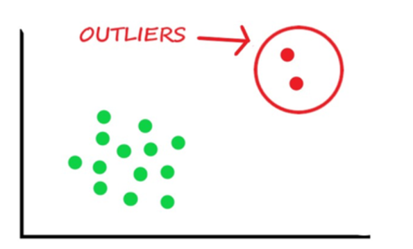
- Strongly affect the mean.
- Increase variability.
- Influence statistical conclusions.
- Indicate unusual events or possible recording errors.
There is no single definition of an outlier.
Statisticians use several methods to identify potential outliers.
Two common methods used in AP Statistics are:
- The IQR Method
- The Standard Deviation Method
1.7.D.1 Methods for Identifying Potential Outliers
A potential outlier is a value that lies unusually far from the center of a distribution according to a specified rule.
The two most common rules are:
- The 1.5 × IQR Rule
- The 2 Standard Deviations Rule
These rules help identify observations that deserve further investigation.
Being identified as a potential outlier does not necessarily mean that the value should be removed from the data set.
The context of the study should always be considered.
1.7.D.1.i Outliers Using the 1.5 × IQR Rule
One common method for identifying potential outliers uses the interquartile range (IQR).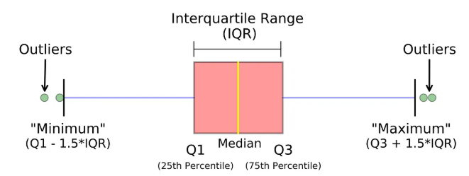
Recall:
\( \mathrm{IQR=Q_3-Q_1} \)
A value is considered a potential outlier if it falls:
- More than \( \mathrm{1.5(IQR)} \) below \( \mathrm{Q_1} \)
- More than \( \mathrm{1.5(IQR)} \) above \( \mathrm{Q_3} \)
Lower Fence Formula
\( \mathrm{Lower\ Fence=Q_1-1.5(IQR)} \)
Upper Fence Formula
\( \mathrm{Upper\ Fence=Q_3+1.5(IQR)} \)
Any observation outside these fences is classified as a potential outlier.
| Condition | Potential Outlier? |
|---|---|
| Below Lower Fence | Yes |
| Above Upper Fence | Yes |
| Between Fences | No |
Example
A data set has: \( \mathrm{Q_1=20} \) and \( \mathrm{Q_3=40} \)
Determine whether: \( \mathrm{75} \) is a potential outlier using the 1.5 × IQR rule.
▶️ Answer / Explanation
Step 1: Calculate the IQR.
\( \mathrm{IQR=40-20=20} \)
Step 2: Calculate the fences.
Lower Fence:
\( \mathrm{20-1.5(20)=-10} \)
Upper Fence:
\( \mathrm{40+1.5(20)=70} \)
Step 3: Compare the value to the fences.
\( \mathrm{75>70} \)
Therefore:
\( \mathrm{75} \)
lies above the upper fence and is a potential outlier.
1.7.D.1.ii Outliers Using the Standard Deviation Rule
Another common method identifies potential outliers using the mean and standard deviation.
A value may be considered a potential outlier if it is more than: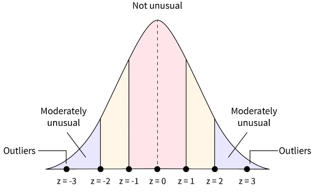
\( \mathrm{2} \)
standard deviations above or below the mean.
Lower Boundary Formula
\( \mathrm{\bar{x}-2s} \)
Upper Boundary Formula
\( \mathrm{\bar{x}+2s} \)
where:
- \( \mathrm{\bar{x}} \) = sample mean
- \( \mathrm{s} \) = sample standard deviation
Values outside these boundaries may be classified as potential outliers.
| Condition | Potential Outlier? |
|---|---|
| Below \( \mathrm{\bar{x}-2s} \) | Yes |
| Above \( \mathrm{\bar{x}+2s} \) | Yes |
| Between the Boundaries | No |
Example
A sample has: \( \mathrm{\bar{x}=50} \) and \( \mathrm{s=8} \)
Determine whether: \( \mathrm{70} \)
is a potential outlier using the standard deviation rule.
▶️ Answer / Explanation
Step 1: Calculate the boundaries.
Lower Boundary:
\( \mathrm{50-2(8)=34} \)
Upper Boundary:
\( \mathrm{50+2(8)=66} \)
Step 2: Compare the value to the boundaries.
\( \mathrm{70>66} \)
Therefore:
\( \mathrm{70} \)
is more than two standard deviations above the mean and is considered a potential outlier.
1.7.E Compare Multiple Quantitative One-Variable Summary Statistics
Statisticians often compare two or more quantitative data sets to identify similarities and differences.
Rather than examining every individual observation, summary statistics provide a concise way to compare distributions.
When comparing quantitative data sets, statisticians focus on:
- Center
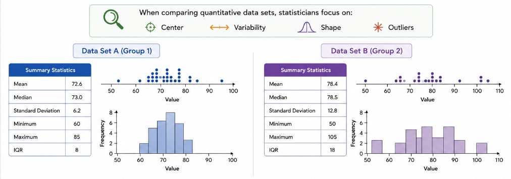
- Variability
- Shape
- Outliers
Comparisons should always be made in context.
For example:
- Which group has the higher typical value?
- Which group is more consistent?
- Which group has greater spread?
- Does one group contain unusual observations?
Summary statistics provide evidence that helps answer these questions.
1.7.E.1 Comparing Quantitative Data Using Summary Statistics
Summary statistics can be used to compare features of two or more independent samples.
Four important features should be considered:
- Center
- Variability
- Shape
- Outliers
1. Comparing Center
Measures of center describe the typical value of a distribution.
Common measures:
- Mean (\( \bar{x} \))
- Median
A larger mean or median indicates a higher typical value.
Example:
- Mean score of Class A = \( \mathrm{82} \)
- Mean score of Class B = \( \mathrm{76} \)
Class A performed better on average.
2. Comparing Variability
Measures of variability describe how spread out the data are.
Common measures:
- Range
- IQR
- Standard Deviation
A larger measure indicates greater variability.
Example:
- IQR of Class A = \( \mathrm{8} \)
- IQR of Class B = \( \mathrm{20} \)
Class B’s scores are more spread out.
3. Comparing Shape
Distributions may differ in shape.
Possible descriptions include:
- Symmetric
- Skewed Right
- Skewed Left
- Unimodal
- Bimodal
- Uniform
Shape comparisons often come from graphical displays such as histograms or dotplots.
4. Comparing Outliers
One distribution may contain outliers while another does not.
Outliers can affect:
- Mean
- Range
- Standard deviation
When comparing distributions, always mention any unusual observations.
| Feature | Summary Statistics Used |
|---|---|
| Center | Mean, Median |
| Variability | Range, IQR, Standard Deviation |
| Shape | Histogram, Dotplot, Stem-and-Leaf Plot |
| Outliers | IQR Rule or Standard Deviation Rule |
AP Statistics Comparison Template
When comparing two distributions, AP Statistics students should discuss:
- Center
- Spread
- Shape
- Outliers
This is often remembered as:
CSSO
- Center
- Spread
- Shape
- Outliers
A complete AP response should address all four characteristics whenever possible.
Example
Two classes took the same mathematics exam.
| Statistic | Class A | Class B |
|---|---|---|
| Mean | 84 | 78 |
| Median | 85 | 77 |
| IQR | 10 | 18 |
| Standard Deviation | 6 | 12 |
Compare the performance of the two classes using the summary statistics.
▶️ Answer / Explanation
Center:
Class A has a higher mean (\( \mathrm{84} \)) and median (\( \mathrm{85} \)) than Class B.
Therefore, Class A performed better overall.
Variability:
Class B has a larger IQR (\( \mathrm{18} \)) and a larger standard deviation (\( \mathrm{12} \)).
Therefore, Class B’s scores are more spread out and less consistent.
Shape:
The shape cannot be determined from the summary statistics alone.
A graphical display would be needed.
Outliers:
No information about outliers is provided.
Based on the available summary statistics, Class A performed better and showed more consistency than Class B.
1.7.F Justify the Selection of a Summary Statistic for Describing Quantitative Data
Different summary statistics provide different information about a quantitative distribution.
The choice of which summary statistic to use depends on the shape of the distribution and the presence of outliers.
Some statistics are strongly affected by unusual observations, while others remain relatively unchanged.
When selecting summary statistics, statisticians consider:
- The shape of the distribution
- The presence of outliers
- The purpose of the analysis
Choosing appropriate summary statistics helps provide an accurate description of the data.
1.7.F.1 Resistant and Nonresistant Statistics
- A resistant (robust) statistic is not greatly affected by unusually large or unusually small observations.
- A nonresistant (non-robust) statistic can change substantially when outliers are present.
Understanding which statistics are resistant is important because outliers can sometimes distort the description of a distribution.
Resistant Measures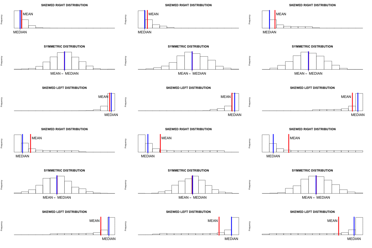
The following statistics are considered resistant:
- Median
- Interquartile Range (IQR)
These statistics depend primarily on the position of observations rather than their actual magnitudes.
As a result, extreme values have little effect on them.
Nonresistant Measures
The following statistics are considered nonresistant:
- Mean
- Range
- Standard Deviation
These statistics use the actual numerical values of the observations.
Therefore, extreme observations can significantly affect their values.
| Statistic | Resistant? | Reason |
|---|---|---|
| Median | Yes | Based on position of values |
| IQR | Yes | Uses quartiles rather than extreme values |
| Mean | No | Uses every value directly |
| Range | No | Depends entirely on minimum and maximum |
| Standard Deviation | No | Uses squared deviations from the mean |
Choosing the Appropriate Summary Statistics
For distributions that are:
- Symmetric
- Without significant outliers
the preferred measures are:
- Mean
- Standard Deviation
For distributions that are:
- Skewed
- Contain outliers
the preferred measures are:
- Median
- IQR
This is one of the most commonly tested concepts in AP Statistics.
| Distribution Type | Preferred Measure of Center | Preferred Measure of Spread |
|---|---|---|
| Symmetric, No Outliers | Mean | Standard Deviation |
| Skewed or Contains Outliers | Median | IQR |
Example
A distribution of household incomes is strongly skewed right because a small number of households earn extremely large incomes.
Which measures of center and variability should be used to describe this distribution?
▶️ Answer / Explanation
Because the distribution is skewed right, the mean and standard deviation may be heavily influenced by the extremely large incomes.
Therefore, the preferred measures are:
- Median (center)
- IQR (spread)
These measures are resistant to outliers and provide a more accurate description of the typical household income.
1.7.F.2 Using Summary Statistics to Justify Claims in Context
Summary statistics provide numerical evidence that can be used to support claims about a quantitative variable.
Rather than making conclusions based on opinion, statisticians use measures such as:
- Mean
- Median
- Range
- IQR
- Standard Deviation
to justify statements about a distribution.
Claims may involve:
- Typical values
- Variability
- Consistency
- Comparisons between groups
A strong statistical justification should:
- Reference specific summary statistics.
- Interpret those statistics in context.
- Connect the evidence directly to the claim.
Weak Claim:
“Class A did better.”
Strong Claim:
“Class A performed better because its median exam score was higher than Class B’s median exam score.”
| Statistic | Possible Claim Supported |
|---|---|
| Mean or Median | Typical value is larger or smaller |
| IQR | Middle 50% is more or less spread out |
| Standard Deviation | Data are more or less consistent |
Example
Two basketball teams recorded the following median points scored per game:
- Team A: \( \mathrm{82} \)
- Team B: \( \mathrm{75} \)
Use the summary statistics to justify a claim about the teams’ scoring performances.
▶️ Answer / Explanation
Team A has a higher median score than Team B.
The median represents the middle score in each distribution.
Since:
\( \mathrm{82>75} \)
Team A typically scores more points per game than Team B.
Therefore, the summary statistics support the claim that Team A generally has stronger scoring performance.