Graphical Representations of Summary Statistics
Graphical displays provide a visual summary of the center, spread, and unusual features of a quantitative distribution. The most common are boxplots (also known as box-and-whisker plots). These rely directly on summary statistics such as the median, quartiles, IQR, and outliers.
Boxplot (Box-and-Whisker Plot)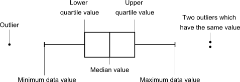
- Constructed using the five-number summary: Minimum, \(Q_1\), Median, \(Q_3\), Maximum.
- A box is drawn from \(Q_1\) to \(Q_3\) with a line at the median.
- Whiskers extend to the minimum and maximum values (unless there are outliers).
Shows skewness:
- Median closer to \(Q_1\) → skewed right.
- Median closer to \(Q_3\) → skewed left.
- Median in middle of box, whiskers about equal length → symmetric.
Modified Boxplot
- Uses the same five-number summary but also identifies outliers.
- Outliers are values beyond \(Q_1 – 1.5 \times IQR\) or \(Q_3 + 1.5 \times IQR\).
- Whiskers extend only to the most extreme non-outlier values.
- Outliers are plotted separately as individual points (often with circles or asterisks).
Side-by-Side Boxplots
- Multiple boxplots drawn on the same scale.
- Used to compare the center, spread, and shape of two or more groups.
- Helpful for comparing treatment vs control, male vs female, before vs after, etc.
Advantages of Boxplots
- Summarize large datasets quickly with key statistics.
- Show spread, center, skewness, and potential outliers.
- Effective for comparing multiple groups.
Limitations
- Do not display the actual shape of the distribution (no info on modality or exact frequencies).
- Less informative than histograms for detailed distribution analysis.
Example
Data (weights in kg) for 12 small packages:
4, 5, 7, 8, 9, 10, 11, 12, 13, 14, 20, 35
Construct a modified boxplot and identify any outliers. Give the five-number summary, IQR, outlier cutoffs, and state where the whiskers should extend.
▶️ Answer / Explanation
Step 1 — Order and five-number summary
- Ordered data: 4, 5, 7, 8, 9, 10, 11, 12, 13, 14, 20, 35.
- Minimum = 4.
- Maximum = 35.
- Median (middle of 12 values) = average of 6th and 7th = \( \dfrac{10 + 11}{2} = 10.5 \).
- \( Q_1 \) = median of lower half (first 6): average of 3rd and 4th = \( \dfrac{7+8}{2} = 7.5 \).
- \( Q_3 \) = median of upper half (last 6): average of 3rd and 4th = \( \dfrac{13+14}{2} = 13.5 \).
- Five-number summary: Min = 4, \(Q_1 = 7.5\), Median = \(10.5\), \(Q_3 = 13.5\), Max = 35.
Step 2 — IQR and outlier cutoffs
- \( IQR = Q_3 – Q_1 = 13.5 – 7.5 = 6 \).
- Lower cutoff: \( Q_1 – 1.5 \times IQR = 7.5 – 1.5(6) = 7.5 – 9 = -1.5 \).
- Upper cutoff: \( Q_3 + 1.5 \times IQR = 13.5 + 1.5(6) = 13.5 + 9 = 22.5 \).
- Any value \(< -1.5\) or \(> 22.5\) is an outlier. In this set, 35 \(>\) 22.5, so 35 is an outlier. All other values are non-outliers.
Step 3 — Whiskers and modified boxplot construction
- Whiskers extend to the most extreme non-outlier values: min non-outlier = 4, max non-outlier = 20.
- Plot a box from \(Q_1 = 7.5\) to \(Q_3 = 13.5\); draw a line at the median \(10.5\). Whiskers from 4 to 20. Mark 35 as an individual outlier point.
Interpretation:
- Shape: Slight right skew because of a long whisker to the right and a high outlier (35).
- Outliers: 35 is an outlier by the IQR rule.
- Center: Median = \(10.5\) kg (typical package weight).
- Spread: IQR = 6 kg (middle 50% between 7.5 and 13.5). Overall range = \(35 – 4 = 31\) kg, but the modified boxplot clarifies that the bulk is between 4 and 20 kg.
Example
Two promotion groups’ weekly sales (in units) were recorded:
Group A: 55, 58, 60, 62, 63, 65, 66, 68, 70, 75
Group B: 45, 48, 50, 52, 53, 55, 57, 59, 60, 200
For each group compute a five-number summary, IQR, and outliers using the IQR rule. Then describe and compare the two distributions with emphasis on center, spread, skewness, and outliers (SOCS). State what a side-by-side boxplot would reveal.
▶️ Answer / Explanation
Group A calculations
- Ordered: 55, 58, 60, 62, 63, 65, 66, 68, 70, 75 (n = 10).
- Median = average of 5th & 6th = \( \dfrac{63 + 65}{2} = 64 \).
- \( Q_1 \) = median of lower half (first 5): 55, 58, 60, 62, 63 → \( Q_1 = 60 \).
- \( Q_3 \) = median of upper half (last 5): 65, 66, 68, 70, 75 → \( Q_3 = 68 \).
- Five-number summary: Min = 55, \(Q_1 = 60\), Median = 64, \(Q_3 = 68\), Max = 75.
- \( IQR = 68 – 60 = 8 \).
- Outlier cutoffs: lower = \(60 – 1.5(8) = 60 – 12 = 48\); upper = \(68 + 1.5(8) = 68 + 12 = 80\). No values \(<48\) or \(>80\), so Group A has no outliers.
Group B calculations
- Ordered: 45, 48, 50, 52, 53, 55, 57, 59, 60, 200 (n = 10).
- Median = average of 5th & 6th = \( \dfrac{53 + 55}{2} = 54 \).
- \( Q_1 \) = median of lower half (first 5): 45, 48, 50, 52, 53 → \( Q_1 = 50 \).
- \( Q_3 \) = median of upper half (last 5): 55, 57, 59, 60, 200 → \( Q_3 = 59 \).
- Five-number summary: Min = 45, \(Q_1 = 50\), Median = 54, \(Q_3 = 59\), Max = 200.
- \( IQR = 59 – 50 = 9 \).
- Outlier cutoffs: lower = \(50 – 1.5(9) = 50 – 13.5 = 36.5\); upper = \(59 + 1.5(9) = 59 + 13.5 = 72.5\). Value 200 \(>\) 72.5, so 200 is a clear outlier; the rest are non-outliers.
Comparison and interpretation (SOCS)
- Shape:
- Group A is roughly symmetric (whiskers and box fairly balanced).
- Group B is strongly right-skewed because of the very large outlier (200) that stretches the right tail.
- Outliers: Group A: none. Group B: 200 is an outlier (IQR rule).
- Center: Group A median = 64 units. Group B median = 54 units. Thus the typical sale is higher in Group A than in Group B.
- Spread:
- Group A IQR = 8, range = \(75 – 55 = 20\).
- Group B IQR = 9, but the overall range \(200 – 45 = 155\) is huge because of the outlier. Ignoring the outlier, Group B’s bulk (non-outlier max = 60) is comparable to Group A but slightly lower.
What a side-by-side boxplot would show
- Two boxes on the same scale: Group A’s box centered higher (median 64) and compact; Group B’s box centered lower (median 54) with a similarly sized IQR but an isolated point far to the right marking the outlier 200.
- Visual takeaway: Group A generally achieves higher weekly sales; Group B has one extreme week (200) that inflates its range and would distort mean-based comparisons. For comparing centers, medians are more informative here.