
2.10.A.1 Binomial Random Variable
A binomial random variable is a discrete random variable that counts the number of successes in a fixed number of repeated independent trials.
Each trial has only two possible outcomes: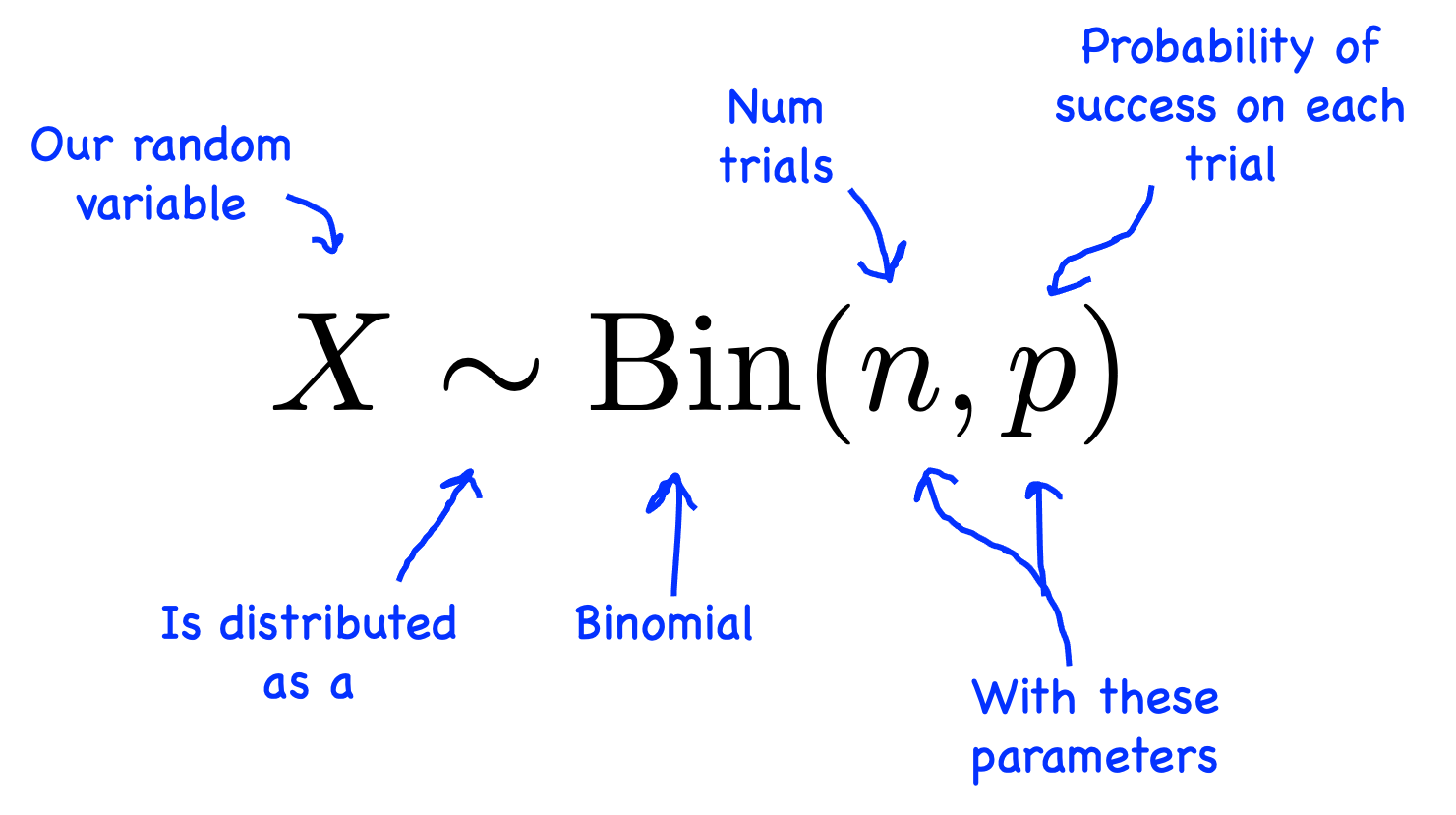
- Success
- Failure
The probability of success remains constant for every trial.
Definition
A random variable \(X\) is a binomial random variable if it counts the number of successes in
- a fixed number of trials (\(n\)),
- that are independent,
- with only two possible outcomes (success or failure),
- where the probability of success is \(p\) and the probability of failure is \(1-p\)
The Four Binomial Conditions (BINS)
| Condition | Meaning |
|---|---|
| B — Binary Outcomes | Each trial has only two possible outcomes: success or failure. |
| I — Independent Trials | The outcome of one trial does not affect another. |
| N — Number of Trials Fixed | The number of trials, \(n\), is fixed before the experiment begins. |
| S — Same Probability of Success | The probability of success, \(p\), is the same for every trial. |
Examples of Binomial Random Variables
Example 1: Coin Tosses
A fair coin is tossed 10 times.
Let
\(X=\) Number of Heads.
This is a binomial random variable because:
- There are 10 fixed trials.
- Each toss has two outcomes (Head or Tail).
- The tosses are independent.
- The probability of Head is always
\(p=\frac12\)
Example 2: Multiple-Choice Test
A student guesses on 20 true/false questions.
Let
\(X=\) Number of correct answers.
This is a binomial random variable because:
- 20 fixed questions.
- Each question has two outcomes (correct or incorrect).
- Each guess is independent.
- The probability of a correct answer is
\(p=\frac12\)
Examples That Are Not Binomial
Example 1
A die is rolled repeatedly until the first 6 appears.
Not binomial because the number of trials is not fixed.
Example 2
A deck of cards is dealt without replacement, and \(X\) is the number of Hearts.
Not binomial because the probability of success changes after each card is removed.
How to Determine if a Random Variable is Binomial
- Is the number of trials fixed?
- Does each trial have only two outcomes?
- Are the trials independent?
- Is the probability of success constant?
If the answer to all four questions is YES, then the random variable is binomial.
Summary of Binomial Conditions
| Requirement | Must Be True? |
|---|---|
| Fixed number of trials | Yes |
| Two outcomes per trial | Yes |
| Independent trials | Yes |
| Constant probability of success | Yes |
| Random variable counts successes | Yes |
Important AP Exam Notes
- A binomial random variable counts the number of successes, not failures.
- Memorize the BINS conditions:
- B – Binary outcomes
- I – Independent trials
- N – Fixed Number of trials
- S – Same probability of success
- If any one of the four conditions is not satisfied, the random variable is not binomial.
- For sampling without replacement, independence is approximately satisfied if the population is at least 10 times the sample size (10% condition).
Common AP Exam Mistakes
| Incorrect | Correct |
|---|---|
| Thinking every random variable is binomial. | All four BINS conditions must be satisfied. |
| Ignoring changing probabilities when sampling without replacement. | The probability of success must remain constant (or approximately constant under the 10% condition). |
| Counting something other than successes. | A binomial random variable always counts successes. |
| Using an experiment that stops after the first success. | A binomial experiment requires a fixed number of trials. |
Example
A basketball player takes 15 free throws. Let \(X\) represent the number of successful free throws.
Determine whether \(X\) is a binomial random variable. Justify your answer.
▶️ Answer / Explanation
Check the BINS conditions:
- B: Two outcomes (make or miss).
- I: Assume the shots are independent.
- N: There are 15 fixed shots.
- S: The probability of making each free throw is assumed to remain constant.
Since all four conditions are satisfied, \(X\) is a binomial random variable.
2.10.B Mean and Standard Deviation of a Binomial Distribution
If a random variable is binomial, its mean and standard deviation can be calculated directly using formulas based on the number of trials and the probability of success.
Suppose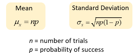
- \(n\) = Number of trials
- \(p\) = Probability of success on each trial
- \(1-p\) = Probability of failure on each trial
Formula
Mean (Expected Value)
\(\mu_X=np\)
Standard Deviation
\(\sigma_X=\sqrt{np(1-p)}\)
Meaning of the Symbols
| Symbol | Meaning |
|---|---|
| \(n\) | Number of independent trials. |
| \(p\) | Probability of success. |
| \(1-p\) | Probability of failure. |
| \(\mu_X\) | Mean (expected number of successes). |
| \(\sigma_X\) | Standard deviation (spread of the number of successes). |
Example 1: Coin Tosses
A fair coin is tossed 20 times.
Let
\(X=\) Number of Heads.
Here,
\(n=20\)
\(p=\frac12=0.5\)
Mean
\(\mu_X=np=(20)(0.5)=10\)
Standard Deviation
\(\sigma_X=\sqrt{20(0.5)(0.5)}=\sqrt5\approx2.24\)
Interpretation
- On average, about 10 Heads are expected in 20 tosses.
- The number of Heads typically differs from 10 by about 2.24 Heads.
Example 2: Free Throws
A basketball player makes a free throw with probability
\(p=0.80\)
The player attempts 15 free throws.
Let
\(X=\) Number of successful free throws.
Step 1: Identify \(n\) and \(p\).
\(n=15,\qquad p=0.80\)
Step 2: Calculate the mean.
\(\mu_X=(15)(0.80)=12\)
Step 3: Calculate the standard deviation.
\(\sigma_X=\sqrt{15(0.80)(0.20)}=\sqrt{2.4}\approx1.55\)
How to Calculate the Mean and Standard Deviation
- Verify that the random variable is binomial (BINS conditions).
- Identify \(n\) and \(p\).
- Use
\(\mu_X=np\)
- Use
\(\sigma_X=\sqrt{np(1-p)}\)
- Interpret the results in context.
Summary Table
| Quantity | Formula | Interpretation |
|---|---|---|
| Mean | \(\mu_X=np\) | Expected number of successes. |
| Standard Deviation | \(\sigma_X=\sqrt{np(1-p)}\) | Typical distance from the expected number of successes. |
Important AP Exam Notes
- These formulas can only be used if the random variable is binomial.
- The mean represents the expected number of successes.
- The standard deviation measures the variability in the number of successes.
- Always identify \(n\) and \(p\) before substituting into the formulas.
- The standard deviation uses both the probability of success, \(p\), and the probability of failure, \(1-p\).
Common AP Exam Mistakes
| Incorrect | Correct |
|---|---|
| Using the formulas without checking that the distribution is binomial. | Verify the BINS conditions first. |
| Using \(p\) instead of \(1-p\) in the standard deviation formula. | Use both \(p\) and \(1-p\). |
| Forgetting the square root when calculating the standard deviation. | Take the square root of \(np(1-p)\). |
| Interpreting the mean as the outcome of one trial. | The mean is the expected number of successes over many repetitions. |
Example
A factory produces light bulbs, and each bulb has a 5% chance of being defective. A quality inspector randomly selects 40 bulbs.
Let \(X\) be the number of defective bulbs selected.
Calculate the mean and standard deviation of the binomial distribution.
▶️ Answer / Explanation
Step 1: Identify the parameters.
\(n=40,\qquad p=0.05\)
Step 2: Calculate the mean.
\(\mu_X=np=(40)(0.05)=2\)
Step 3: Calculate the standard deviation.
\(\sigma_X=\sqrt{40(0.05)(0.95)}=\sqrt{1.9}\approx1.38\)
Answer
- Mean: \(\mu_X=2\) defective bulbs.
- Standard deviation: \(\sigma_X\approx1.38\) defective bulbs.
2.10.D Estimating Probabilities of Binomial Random Variables Using Simulations
A binomial probability distribution can be obtained in two ways:
- Using the rules of probability (exact probabilities).
- Using a simulation (estimated probabilities).
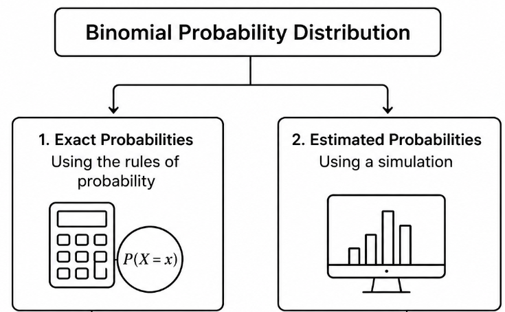
When calculating exact probabilities is difficult or when a computer simulation is available, a simulation can be used to estimate the probabilities of a binomial random variable.
What is a Simulation?
A simulation is a method of using random outcomes to imitate a real-world random process.
For a binomial experiment, each simulation consists of:
- A fixed number of independent trials.
- Each trial having two possible outcomes (success or failure).
- The same probability of success for every trial.
After many repetitions, the relative frequencies of the outcomes are used to estimate the probabilities.
Estimating Probability from a Simulation
The estimated probability of an event is
\(\text{Estimated Probability}=\dfrac{\text{Number of Times the Event Occurred}}{\text{Total Number of Simulation Trials}}\)
As the number of simulation trials increases, the estimated probability generally becomes closer to the true probability.
Example 1: Tossing Coins
A fair coin is tossed 5 times.
Let
\(X=\) Number of Heads obtained.
A computer performs 2,000 simulations.
Suppose the simulation produces exactly 3 Heads in 630 trials.
The estimated probability is
\(P(X=3)\approx\dfrac{630}{2000}=0.315\)
Interpretation
Based on the simulation, there is approximately a 31.5% chance of obtaining exactly 3 Heads when a fair coin is tossed five times.
Example 2: Free Throws
A basketball player makes a free throw with probability
\(p=0.80\)
The player attempts 10 free throws.
Suppose a simulation of 5,000 experiments shows that the player makes at least 8 free throws in 3,395 experiments.
The estimated probability is
\(P(X\ge8)\approx\dfrac{3395}{5000}=0.679\)
Interpretation
Based on the simulation, there is approximately a 67.9% chance that the player makes at least 8 free throws out of 10 attempts.
Steps for Using a Simulation
- Identify the binomial experiment.
- Repeat the experiment many times using random numbers or technology.
- Record the number of successes for each repetition.
- Count how many simulations satisfy the event of interest.
- Estimate the probability using the relative frequency.
Simulation vs. Exact Probability
| Exact Probability | Simulation |
|---|---|
| Calculated using probability rules. | Estimated using repeated random trials. |
| Produces the true probability. | Produces an approximation of the true probability. |
| No random error. | Subject to random variation. |
| Useful when formulas are available. | Useful when exact calculations are difficult. |
Relationship to the Law of Large Numbers
The Law of Large Numbers explains why simulations work.
As the number of simulation trials becomes very large, the relative frequency of an event approaches its true probability.
Important AP Exam Notes
- A simulation estimates probabilities using relative frequencies.
- More simulation trials generally produce a more accurate estimate of the true probability.
- Simulation results will vary slightly from one experiment to another because of random variation.
- On the AP Exam, interpret simulated probabilities in the context of the problem.
- Simulations are especially useful when exact probability calculations are difficult or unavailable.
Common AP Exam Mistakes
| Incorrect | Correct |
|---|---|
| Treating a simulated probability as the exact probability. | Simulation provides an estimate of the probability. |
| Using too few simulation trials to make strong conclusions. | Larger numbers of trials produce better estimates. |
| Ignoring the context when interpreting the result. | Always describe the probability using the situation in the problem. |
| Forgetting to divide by the total number of simulations. | Estimated probability = Successful simulations ÷ Total simulations. |
Example
A factory produces electronic chips. Each chip has a 10% chance of being defective.
A simulation of 10,000 samples, each containing 8 chips, is performed.
In the simulation, exactly 2 defective chips occurred in 1,499 samples.
Estimate the probability that exactly two chips are defective, and interpret the result.
▶️ Answer / Explanation
Step 1: Calculate the estimated probability.
\(P(X=2)\approx\dfrac{1499}{10000}=0.1499\)
Step 2: Interpret the result.
Based on the simulation, there is approximately a 15.0% chance that a random sample of 8 chips contains exactly 2 defective chips.
2.10.E.1 Calculating Probabilities for a Binomial Distribution
If a random variable follows a binomial distribution, the probability of obtaining exactly \(x\) successes in \(n\) independent trials can be calculated using the binomial probability formula.
The probability of obtaining exactly \(x\) successes is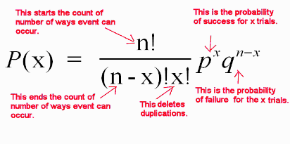
\( \mathrm{ P(X=x)=\binom{n}{x}p^x(1-p)^{\,n-x} }\)
Where:
- \(X\) = Binomial random variable.
- \(x\) = Number of successes.
- \(n\) = Total number of independent trials.
- \(p\) = Probability of success on each trial.
- \(1-p\) = Probability of failure on each trial.
- \(\binom{n}{x}\) = Number of ways to choose \(x\) successes from \(n\) trials.
The possible values of the random variable are
\(x=0,1,2,\ldots,n\)
Meaning of the Formula
The binomial probability formula combines three parts:
| Part of Formula | Meaning |
|---|---|
| \(\binom{n}{x}\) | Number of different ways the successes can occur. |
| \(p^x\) | Probability of obtaining the required number of successes. |
| \((1-p)^{n-x}\) | Probability of obtaining the remaining failures. |
How to Calculate a Binomial Probability
- Verify that the random variable satisfies the BINS conditions.
- Identify \(n\), \(p\), and \(x\).
- Substitute the values into the binomial probability formula.
- Evaluate using a calculator or statistical technology.
Example 1: Coin Tosses
A fair coin is tossed 4 times.
Let
\(X=\) Number of Heads.
Find
\(P(X=2)\)
Step 1: Identify the values.
\(n=4,\qquad x=2,\qquad p=0.5\)
Step 2: Substitute into the formula.
\( P(X=2)=\binom42(0.5)^2(0.5)^2 \)
Step 3: Calculate.
\( =\;6(0.25)(0.25) =6(0.0625) =0.375 \)
Answer
There is a 37.5% probability of obtaining exactly 2 Heads.
Example 2: Free Throws
A basketball player makes a free throw with probability
\(p=0.80\)
The player attempts 5 free throws.
Find the probability that the player makes exactly 4 shots.
Step 1:
\(n=5,\qquad x=4,\qquad p=0.80\)
Step 2:
\( P(X=4)=\binom54(0.80)^4(0.20)^1 \)
Step 3:
\( =5(0.4096)(0.20) =0.4096 \)
Interpretation
There is approximately a 40.96% chance that the player makes exactly 4 of the 5 free throws.
Summary Table
| Symbol | Meaning |
|---|---|
| \(n\) | Number of trials. |
| \(x\) | Number of successes. |
| \(p\) | Probability of success. |
| \(1-p\) | Probability of failure. |
| \(\binom{n}{x}\) | Number of possible arrangements of the successes. |
Important AP Exam Notes
- The binomial probability formula calculates the probability of exactly \(x\) successes.
- The random variable can only take values
\(0,1,2,\ldots,n\)
- Always verify that the random variable satisfies the BINS conditions before using the formula.
- On the AP Exam, binomial probabilities are typically calculated using a graphing calculator or statistical software, but you should understand what each part of the formula represents.
Common AP Exam Mistakes
| Incorrect | Correct |
|---|---|
| Using the formula without checking the BINS conditions. | Verify the experiment is binomial first. |
| Using the wrong value of \(x\). | \(x\) is the number of successes requested. |
| Using \(p\) for both success and failure. | Use \(p\) for success and \(1-p\) for failure. |
| Confusing “exactly,” “at least,” and “at most.” | The formula directly calculates only exactly \(x\) successes. |
Example
A factory produces electronic chips, and each chip has a 10% chance of being defective.
A quality inspector randomly selects 6 chips.
Find the probability that exactly 2 chips are defective.
▶️ Answer / Explanation
Step 1: Identify the values.
\(n=6,\qquad x=2,\qquad p=0.10\)
Step 2: Apply the binomial formula.
\( P(X=2)=\binom62(0.10)^2(0.90)^4 \)
Step 3: Calculate.
\( =15(0.01)(0.6561) \approx0.0984 \)
Answer: The probability that exactly 2 chips are defective is approximately 0.0984 (9.84%).