
2.11.A.1 Continuous Random Variable
A continuous random variable is a variable that can take any numerical value within a specified interval or domain.
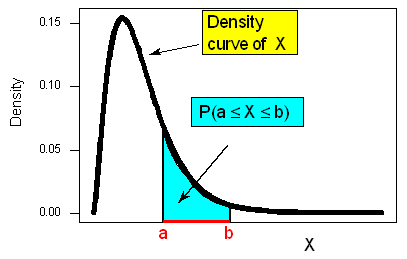
- Unlike a discrete random variable, which takes only specific countable values, a continuous random variable can assume infinitely many possible values within its range.
- Instead of assigning probability to a single value, probabilities are assigned to intervals of values.
- Every interval within the domain has an associated probability.
Examples of Continuous Random Variables
| Continuous Random Variable | Possible Values |
|---|---|
| Height of a student | 170.1 cm, 170.15 cm, 170.152 cm, … |
| Time to complete a race | 9.82 s, 9.821 s, 9.8215 s, … |
| Body temperature | 36.8°C, 36.81°C, 36.812°C, … |
Continuous vs. Discrete Random Variables
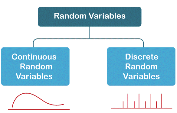
| Continuous | Discrete |
|---|---|
| Can take any value within an interval. | Can take only specific countable values. |
| Usually measured. | Usually counted. |
Important AP Exam Notes
- A continuous random variable can take any value within a specified interval.
- Probabilities are assigned to intervals, not individual values.
- Many continuous random variables are modeled using the normal distribution.
Example
Determine whether each variable is continuous or discrete.
- Height of students in a class.
- Number of siblings a student has.
▶️ Answer / Explanation
1. Height is a continuous random variable because it can take any value within an interval.
2. Number of siblings is a discrete random variable because it can only take whole-number values.
2.11.A.2 Many Continuous Random Variables Follow a Normal Distribution
Many real-world continuous random variables are well modeled by a normal distribution.
- A normal distribution provides a mathematical model that closely approximates the distribution of many naturally occurring measurements.
- Examples include heights, blood pressure, IQ scores, measurement errors, and standardized test scores.
Examples of Variables Often Modeled by a Normal Distribution
| Variable | Typically Normal? |
|---|---|
| Adult heights | Yes |
| IQ scores | Yes |
| Birth weights | Often |
| Test scores | Sometimes |
Important AP Exam Notes
- Not every continuous variable is normally distributed.
- The normal distribution is a useful model for many real-world measurements.
- Always examine the context before assuming normality.
Example
Which of the following variables is most likely to be modeled by a normal distribution?
- Adult heights
- Number of children in a family
▶️ Answer / Explanation
The correct answer is Adult heights.
Adult heights are continuous measurements and are commonly modeled by a normal distribution.
2.11.A.3 Characteristics of a Normal Distribution
A normal distribution is a continuous probability distribution with a characteristic shape known as the normal curve.
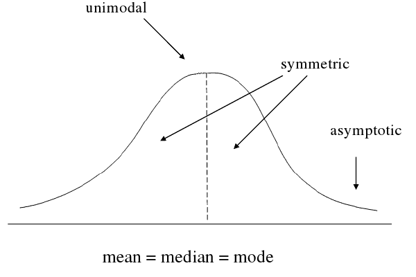
The normal curve has four important characteristics.
| Characteristic | Description |
|---|---|
| Continuous | The curve contains infinitely many possible values. |
| Unimodal | The curve has one peak. |
| Bell-shaped | Most observations are near the center with fewer observations toward the tails. |
| Symmetric | The left and right sides are mirror images about the mean. |
Important AP Exam Notes
- A normal curve is always continuous.
- It has exactly one peak (unimodal).
- The curve is symmetric about the mean.
- The tails extend indefinitely but never touch the horizontal axis.
Example
State four characteristics of a normal distribution.
▶️ Answer / Explanation
- Continuous
- Unimodal
- Bell-shaped
- Symmetric about the mean
2.11.A.4 Using the Normal Curve as a Probability Model
A normal curve can be used to model the distribution of observed data as well as the distribution of a continuous random variable.
When data follow a normal distribution, probabilities can be determined by calculating the area under the normal curve.
- The total area under a normal curve is always equal to \(1\)
- or 100%, representing the probability of the entire sample space.
Applications of the Normal Curve
- Modeling heights and weights.
- Modeling standardized test scores.
- Modeling measurement errors.
- Calculating probabilities for continuous random variables.
- Estimating the proportion of observations within an interval.
Important AP Exam Notes
- The area under the normal curve represents probability.
- The total area under every normal curve equals 1.
- Probabilities correspond to areas over intervals, not single points.
- The normal curve is used to model both data distributions and continuous random variables.
Example
Explain how a normal curve is used to model a continuous random variable.
▶️ Answer / Explanation
A normal curve models the distribution of a continuous random variable by representing probabilities as areas under the curve.
The total area under the curve equals 1, and the area over an interval represents the probability that the variable falls within that interval.
2.11.A.5 Parameters of a Normal Distribution
Every normal distribution is completely described by two parameters:
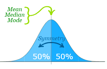
- The population mean, \( \mu \)
- The population standard deviation, \( \sigma \)
The mean determines the center (location) of the normal curve, while the standard deviation determines the spread (variability) of the distribution.
Changing either parameter changes the appearance of the normal curve.
The Two Parameters of a Normal Distribution
| Parameter | Symbol | Role |
|---|---|---|
| Population Mean | \( \mu \) | Determines the center (location) of the normal curve. |
| Population Standard Deviation | \( \sigma \) | Determines the spread (variability) of the normal curve. |
Effect of the Mean (\( \mu \))
The mean determines the center of the distribution.
- Increasing \( \mu \) shifts the entire normal curve to the right.
- Decreasing \( \mu \) shifts the entire normal curve to the left.
- Changing the mean does not change the shape of the curve.
Effect of the Standard Deviation (\( \sigma \))
The standard deviation determines how spread out the data are around the mean.
| Standard Deviation | Appearance of the Normal Curve |
|---|---|
| Small \( \sigma \) | Curve is taller, narrower, and more concentrated around the mean. |
| Large \( \sigma \) | Curve is shorter, wider, and more spread out around the mean. |
As the standard deviation increases, the observations become more dispersed, causing the curve to spread out.
As the standard deviation decreases, the observations become more concentrated near the mean, causing the curve to become taller and narrower.
Important AP Exam Notes
- Every normal distribution is completely determined by two parameters: \( \mu \) and \( \sigma \).
- The mean (\( \mu \)) determines the center of the distribution.
- The standard deviation (\( \sigma \)) determines the spread of the distribution.
- A smaller standard deviation produces a taller and narrower normal curve.
- A larger standard deviation produces a shorter and wider normal curve.
- Changing the mean shifts the curve but does not change its shape.
Common AP Exam Mistakes
| Incorrect Statement | Correct Statement |
|---|---|
| The mean changes the width of the curve. | The mean only changes the location (center). |
| A larger standard deviation makes the curve taller. | A larger standard deviation makes the curve shorter and wider. |
| A smaller standard deviation spreads the data out. | A smaller standard deviation concentrates the data around the mean. |
Example
Two normal distributions have the same mean of \(50\).
- Distribution A has \( \sigma = 4 \).
- Distribution B has \( \sigma = 10 \).
Compare the shapes of the two normal curves.
▶️ Answer / Explanation
Both distributions are centered at 50 because they have the same mean.
Distribution A has a smaller standard deviation, so its curve is taller and narrower, with values more concentrated around the mean.
Distribution B has a larger standard deviation, so its curve is shorter and wider, with values more spread out from the mean.
2.11.B.1 Standard Normal Distribution
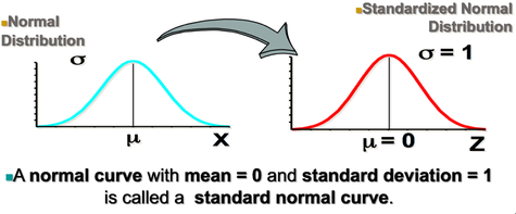
A standard normal distribution is a special type of normal distribution that has:
- A mean of \( \mu = 0 \)
- A standard deviation of \( \sigma = 1 \)
It has the same bell-shaped, symmetric, and continuous shape as every normal distribution, but it is centered at 0 and its spread is measured in units of one standard deviation.
The standard normal distribution is commonly used to calculate probabilities and determine z-scores.
Parameters of the Standard Normal Distribution
| Parameter | Value | Meaning |
|---|---|---|
| Mean | \( \mu = 0 \) | The center of the distribution. |
| Standard Deviation | \( \sigma = 1 \) | The spread of the distribution. |
Characteristics of the Standard Normal Distribution
- Continuous.
- Bell-shaped.
- Symmetric about the mean.
- Unimodal (one peak).
- Mean equals the median and the mode.
- Total area under the curve is 1.
Why Is It Called “Standard”?
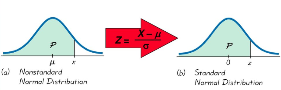
Any normal distribution can be transformed into a standard normal distribution by converting values into z-scores.
This allows statisticians to compare observations from different normal distributions using the same probability model.
The z-score formula is
\( z=\dfrac{x-\mu}{\sigma} \)
where:
- \(x\) = observed value
- \(\mu\) = population mean
- \(\sigma\) = population standard deviation
(The z-score formula will be studied in greater detail later in the course.)
Normal Distribution vs. Standard Normal Distribution
| Normal Distribution | Standard Normal Distribution |
|---|---|
| Can have any mean \( \mu \). | Always has \( \mu = 0 \). |
| Can have any standard deviation \( \sigma \). | Always has \( \sigma = 1 \). |
| Shape depends on \( \mu \) and \( \sigma \). | Always has the same standardized shape. |
Important AP Exam Notes
- The standard normal distribution always has a mean of 0 and a standard deviation of 1.
- It is a special case of the normal distribution.
- It is used to calculate probabilities and interpret z-scores.
- The total area under the standard normal curve is always 1.
- The curve is symmetric about 0.
Common AP Exam Mistakes
| Incorrect Statement | Correct Statement |
|---|---|
| Every normal distribution is standard normal. | Only a normal distribution with \( \mu =0 \) and \( \sigma =1 \) is standard normal. |
| The standard normal distribution has any mean. | Its mean is always \(0\). |
| The standard deviation can vary. | Its standard deviation is always \(1\). |
Example
Determine whether each of the following distributions is a standard normal distribution.
- \( \mu = 0,\; \sigma = 1 \)
- \( \mu = 50,\; \sigma = 10 \)
- \( \mu = 0,\; \sigma = 5 \)
▶️ Answer / Explanation
1. Yes.
It is a standard normal distribution because the mean is 0 and the standard deviation is 1.
2. No.
The mean is not 0 and the standard deviation is not 1.
3. No.
The mean is 0, but the standard deviation is 5 instead of 1.
2.11.C.1 The Empirical Rule (68–95–99.7 Rule)
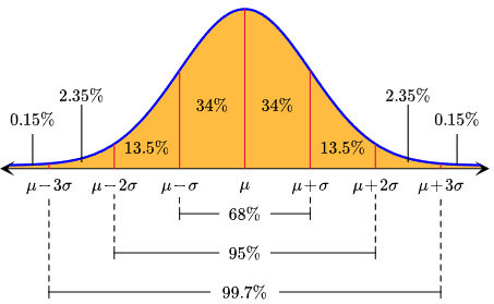
The Empirical Rule, also known as the 68–95–99.7 Rule, is used to estimate the percentage (or probability) of observations that fall within a specified number of standard deviations from the mean in a normal distribution.
- Because a normal distribution is symmetric, the percentages are divided equally on both sides of the mean.
- The Empirical Rule provides a quick way to estimate probabilities without using technology or a normal distribution table.
The Empirical Rule
| Distance from the Mean | Approximate Percentage of Observations |
|---|---|
| Within 1 Standard Deviation (\(\mu \pm 1\sigma\)) | 68% |
| Within 2 Standard Deviations (\(\mu \pm 2\sigma\)) | 95% |
| Within 3 Standard Deviations (\(\mu \pm 3\sigma\)) | 99.7% |
Key Percentages on the Normal Curve
| Region | Approximate Percentage |
|---|---|
| Mean to ±1σ | $34\%$ |
| Between 1σ and 2σ (each side) | $13.5\%$ |
| Between 2σ and 3σ (each side) | $2.35\%$ |
| Beyond 3σ (each tail) | $0.15\%$ |
Example 1
The heights of adult women are approximately normally distributed with
- Mean: \( \mu = 165 \) cm
- Standard Deviation: \( \sigma = 5 \) cm
Estimate the percentage of women whose heights are between 160 cm and 170 cm.
Step 1: Determine the interval.
\(160=165-5=\mu-1\sigma\)
\(170=165+5=\mu+1\sigma\)
Step 2: Apply the Empirical Rule.
Approximately 68% of observations are within one standard deviation of the mean.
Answer: Approximately 68%.
Example 2
Using the same distribution, estimate the percentage of women whose heights are between 155 cm and 175 cm.
\(155=\mu-2\sigma\)
\(175=\mu+2\sigma\)
According to the Empirical Rule, approximately
95%
of observations are within two standard deviations of the mean.
Example 3
Estimate the percentage of women who are taller than 175 cm.
Since 175 cm is 2 standard deviations above the mean,
Within ±2σ = 95%
The remaining probability is
\(100\%-95\%=5\%\)
Because the normal distribution is symmetric,
\( \dfrac{5\%}{2}=2.5\% \)
Answer: Approximately 2.5%.
Important AP Exam Notes
- The Empirical Rule applies only to approximately normal distributions.
- The distribution must be symmetric and bell-shaped.
- Remember the three key percentages:
- 68% within 1 standard deviation.
- 95% within 2 standard deviations.
- 99.7% within 3 standard deviations.
- The normal distribution is symmetric, so divide percentages equally on both sides of the mean.
- Use the Empirical Rule for quick estimates without technology.
Common AP Exam Mistakes
| Incorrect | Correct |
|---|---|
| Applying the Empirical Rule to a skewed distribution. | Use it only for approximately normal distributions. |
| Forgetting to divide tail probabilities equally. | The normal distribution is symmetric. |
| Confusing the 68%, 95%, and 99.7% values. | Memorize the 68–95–99.7 Rule. |
Example
The weights of newborn babies are approximately normally distributed with a mean of 3.4 kg and a standard deviation of 0.5 kg.
Using the Empirical Rule, estimate:
- The percentage of babies weighing between 2.9 kg and 3.9 kg.
- The percentage of babies weighing more than 4.4 kg.
▶️ Answer / Explanation
1.
Since
\(2.9=\mu-1\sigma\)
\(3.9=\mu+1\sigma\)
Approximately
68%
of babies weigh between 2.9 kg and 3.9 kg.
2.
Since
\(4.4=\mu+2\sigma\)
The area beyond +2 standard deviations is
\( \dfrac{100\%-95\%}{2}=2.5\% \)
Approximately 2.5% of babies weigh more than 4.4 kg.
2.11.D.1 Calculating Probability for an Interval of a Normal Distribution
If a random variable follows an approximately normal distribution, then the probability that the variable falls within a particular interval is equal to the area under the normal curve over that interval.
In a normal distribution, probabilities are represented by areas under the curve, not by the heights of the curve.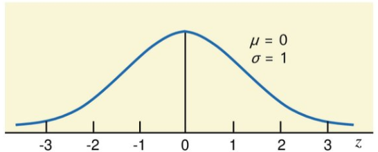
The total area under every normal curve is
\(1\) or $100\%$
This means the probability that a randomly selected observation falls somewhere on the normal curve is always 1.
Key Idea
For a normally distributed random variable \(X\),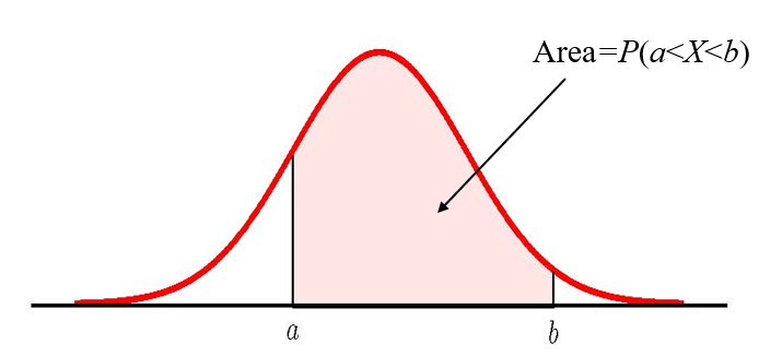
\(P(a \le X \le b)\)
represents the area under the normal curve between the values \(a\) and \(b\).
Similarly,
- \(P(X<a)\) = Area to the left of \(a\).
- \(P(X>a)\) = Area to the right of \(a\).
- \(P(a<X<b)\) = Area between \(a\) and \(b\).
Total Area Under the Normal Curve
| Region | Probability (Area) |
|---|---|
| Entire curve | 1.000 |
| Left of a value | Area to the left of that value. |
| Right of a value | Area to the right of that value. |
| Between two values | Area between the two values. |
Finding Probabilities with Technology
When the mean and standard deviation are known, probabilities for a normal distribution are usually calculated using a graphing calculator or statistical software.
TI-84 Calculator
2nd → VARS (DISTR) → normalcdf(
The command is
normalcdf(lower bound, upper bound, mean, standard deviation)
Example 1
The heights of adult women are approximately normally distributed with
- Mean: \( \mu=165\text{ cm} \)
- Standard deviation: \( \sigma=5\text{ cm} \)
Find the probability that a randomly selected woman has a height between 160 cm and 170 cm.
Technology
normalcdf(160,170,165,5)
Calculator Output
\(P(160<X<170)\approx0.683\)
Interpretation
Approximately 68.3% of adult women have heights between 160 cm and 170 cm.
Example 2
Using the same distribution, find the probability that a randomly selected woman is taller than 175 cm.
Technology
normalcdf(175,1E99,165,5)
Calculator Output
\(P(X>175)\approx0.0228\)
Interpretation
Approximately 2.28% of adult women are taller than 175 cm.
Example 3
Using the same distribution, find the probability that a randomly selected woman is shorter than 158 cm.
Technology
normalcdf(-1E99,158,165,5)
Calculator Output
\(P(X<158)\approx0.0808\)
Interpretation
Approximately 8.08% of adult women are shorter than 158 cm.
Important AP Exam Notes
- For a normal distribution, probabilities are represented by areas under the normal curve.
- The total area under every normal curve is always 1.
- Area to the left = Probability less than a value.
- Area to the right = Probability greater than a value.
- Area between two values = Probability of being within that interval.
- AP Statistics students are expected to use technology (such as a TI-84 calculator) to calculate normal probabilities.
Common AP Exam Mistakes
| Incorrect | Correct |
|---|---|
| Adding probabilities instead of finding the area. | Probability equals the area under the curve. |
| Using the height of the curve as the probability. | Use the area beneath the curve. |
| Using incorrect calculator bounds. | Use the correct lower and upper bounds in normalcdf(). |
Example
The scores on an AP Statistics practice exam are approximately normally distributed with a mean of 75 and a standard deviation of 8.
Using technology, calculate the probability that a randomly selected student scores between 70 and 85.
▶️ Answer / Explanation
Step 1: Identify the values.
- Lower bound = 70
- Upper bound = 85
- Mean = 75
- Standard deviation = 8
Step 2: Calculator command.
normalcdf(70,85,75,8)
Step 3: Calculator output.
\(P(70<X<85)\approx0.628\)
Interpretation
There is approximately a 0.628 probability (or 62.8%) that a randomly selected student scores between 70 and 85.
2.11.E.1 Finding Interval Boundaries for a Given Area in a Normal Distribution
In a normal distribution, the boundaries (cutoff values) that correspond to a given probability or area can be determined using: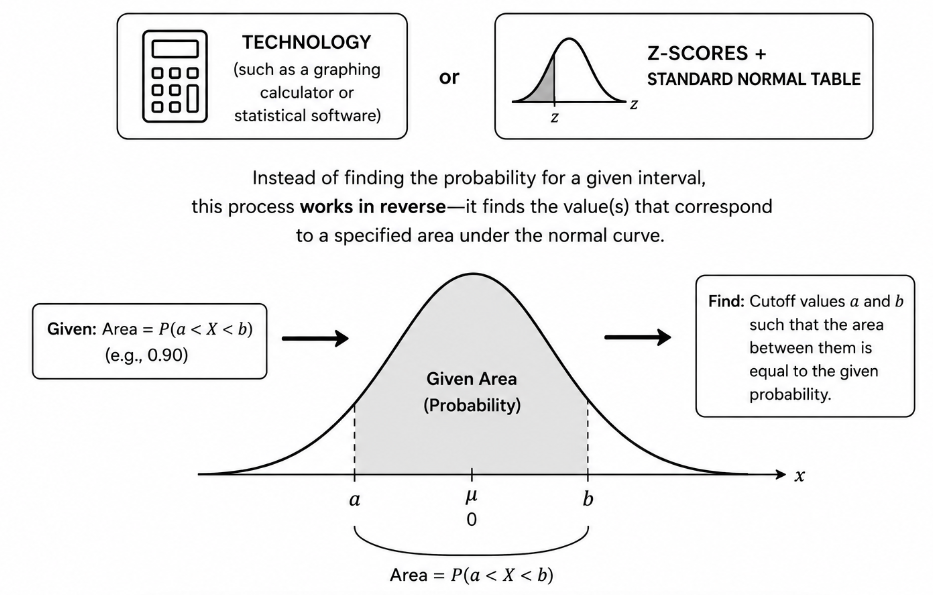
- Technology (such as a graphing calculator or statistical software), or
- z-scores together with a standard normal table.
Instead of finding the probability for a given interval, this process works in reverse , it finds the value(s) that correspond to a specified area under the normal curve.
Key Idea
Since the area under a normal curve represents probability, a specified probability (or percentage) determines one or more cutoff values on the horizontal axis.
These cutoff values define the interval that contains the given area.
Methods for Finding Interval Boundaries
| Method | Description |
|---|---|
| Technology | Uses the calculator’s invNorm() function to determine the boundary value. |
| Standard Normal Table | Find the appropriate z-score from the cumulative area, then convert back to the original scale if necessary. |
Using Technology (TI-84 Calculator)
To find a boundary value, use
2nd → VARS (DISTR) → invNorm(
The syntax is
invNorm(area to the left, mean, standard deviation)
The calculator returns the value that has the specified cumulative area to its left.
Example 1
The heights of adult women are approximately normally distributed with
- Mean: \( \mu=165\text{ cm} \)
- Standard deviation: \( \sigma=5\text{ cm} \)
Find the height that marks the 90th percentile.
Calculator Command
invNorm(0.90,165,5)
Calculator Output
\(173.4\text{ cm}\)
Interpretation
Approximately 90% of adult women are shorter than 173.4 cm, and approximately 10% are taller.
Example 2
The scores on an AP Statistics exam are approximately normally distributed with
- Mean: \(75\)
- Standard deviation: \(8\)
Find the score that separates the lowest 25% of students.
Calculator Command
invNorm(0.25,75,8)
Calculator Output
\(69.6\)
Interpretation
Approximately 25% of students scored below 69.6.
Relationship Between Area and Boundary
| Given Area | Boundary Found |
|---|---|
| Area to the left | Lower percentile cutoff |
| Area to the right | Upper percentile cutoff |
| Middle area | Lower and upper interval boundaries |
Important AP Exam Notes
- Boundary values for a normal distribution can be found using technology or a standard normal table.
- The calculator function invNorm() finds the value associated with a given cumulative probability.
- The probability entered into invNorm() is always the area to the left of the desired value.
- The returned value is the boundary that separates the specified proportion of observations.
- Technology is the primary method used on the AP Statistics Exam.
Common AP Exam Mistakes
| Incorrect | Correct |
|---|---|
| Using normalcdf() to find a boundary. | Use invNorm() to find cutoff values. |
| Entering the area to the right into invNorm(). | Always enter the cumulative area to the left. |
| Confusing probabilities with boundary values. | The area determines the cutoff value on the horizontal axis. |
Example
The weights of newborn babies are approximately normally distributed with a mean of 3.4 kg and a standard deviation of 0.5 kg.
Find the birth weight that marks the 95th percentile.
▶️ Answer / Explanation
Step 1: The 95th percentile means that 95% of observations lie to the left of the desired value.
Step 2: Calculator command
invNorm(0.95,3.4,0.5)
Step 3: Calculator output
\(4.22\text{ kg}\)
Interpretation
Approximately 95% of newborn babies weigh less than 4.22 kg, and approximately 5% weigh more.
2.11.E.2 Determining Intervals for a Given Area in a Normal Distribution
Intervals associated with a specified area (probability) in a normal distribution can be determined by assigning the appropriate inequalities to the boundary values of the interval.
Suppose:
- \(p\) = percentage of observations (where \(0 \le p \le 100\))
- \(x_a\) = lower boundary of the interval
- \(x_b\) = upper boundary of the interval
Depending on the wording of the problem, the interval may describe:
- The lowest \(p\%\) of observations
- The middle \(p\%\) of observations
- The highest \(p\%\) of observations
- The most extreme \(p\%\) of observations (split equally between both tails)
Four Common Types of Probability Intervals
| Description | Probability Statement |
|---|---|
| Lowest \(p\%\) | \(P(X<x_a)=\dfrac{p}{100}\) |
| Middle \(p\%\) | \(P(x_a<X<x_b)=\dfrac{p}{100}\) |
| Highest \(p\%\) | \(P(X>x_b)=\dfrac{p}{100}\) |
| Most Extreme \(p\%\) | \(P(X<x_a)=\dfrac{p}{200}\) and \(P(X>x_b)=\dfrac{p}{200}\) |
1. Lowest \(p\%\) of Observations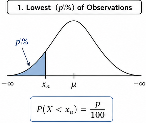
If the problem asks for the lowest \(p\%\) of observations, find the boundary \(x_a\) such that
\(P(X<x_a)=\dfrac{p}{100}\)
Example
Find the value separating the lowest 20% of a normal distribution.
Use
invNorm(0.20,\(\mu\),\(\sigma\))
The returned value is the cutoff below which 20% of observations lie.
2. Middle \(p\%\) of Observations
If the problem asks for the middle \(p\%\), determine two boundary values:
\(P(x_a<X<x_b)=\dfrac{p}{100}\)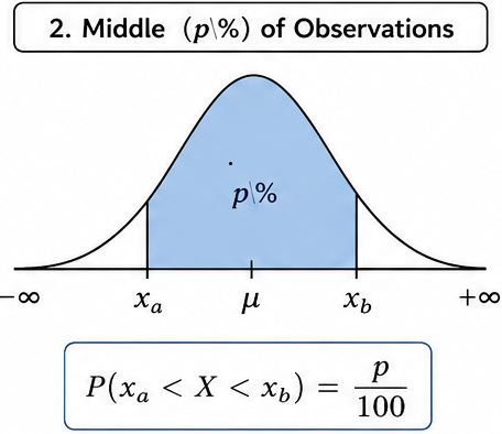
Since the normal distribution is symmetric, the remaining probability is divided equally between the two tails.
Example
Find the interval containing the middle 90%.
Remaining probability:
\(100\%-90\%=10\%\)
Each tail contains
\(5\%\)
Find:
- Lower boundary → invNorm(0.05,\(\mu\),\(\sigma\))
- Upper boundary → invNorm(0.95,\(\mu\),\(\sigma\))
3. Highest \(p\%\) of Observations
If the problem asks for the highest \(p\%\), find the boundary \(x_b\) such that
\(P(X>x_b)=\dfrac{p}{100}\)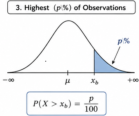
Because invNorm() requires the cumulative area to the left, use
Area to the left = \(1-\dfrac{p}{100}\)
Example
Find the value separating the highest 10%.
Area to the left:
\(1-0.10=0.90\)
Calculator:
invNorm(0.90,\(\mu\),\(\sigma\))
4. Most Extreme \(p\%\) of Observations
If the problem asks for the most extreme \(p\%\), the probability is divided equally between the two tails.
Each tail contains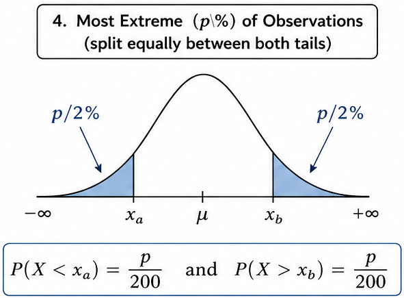
\(\dfrac{p}{200}\)
Therefore,
\(P(X<x_a)=\dfrac{p}{200}\)
and
\(P(X>x_b)=\dfrac{p}{200}\)
Example
Find the cutoff values for the most extreme 4%.
Each tail contains
\(2\%\)
Find
- Lower boundary → invNorm(0.02,\(\mu\),\(\sigma\))
- Upper boundary → invNorm(0.98,\(\mu\),\(\sigma\))
Summary Table
| Question Type | Calculator Area(s) |
|---|---|
| Lowest \(p\%\) | \(p/100\) |
| Highest \(p\%\) | \(1-p/100\) |
| Middle \(p\%\) | Lower = \((1-p/100)/2\) Upper = \(1-(1-p/100)/2\) |
| Most Extreme \(p\%\) | Lower = \(p/200\) Upper = \(1-p/200\) |
Important AP Exam Notes
- Carefully identify whether the question asks for the lowest, highest, middle, or most extreme percentage.
- invNorm() always requires the cumulative area to the left.
- For middle intervals, split the remaining probability equally between the two tails.
- For the most extreme percentages, divide the given percentage equally between both tails.
- Always interpret the resulting boundary values in the context of the problem.
Common AP Exam Mistakes
| Incorrect | Correct |
|---|---|
| Using 0.10 for the highest 10%. | Use 0.90 because invNorm uses left-tail area. |
| Forgetting to split the remaining area for middle intervals. | Divide the remaining probability equally between both tails. |
| Not dividing the extreme percentage between two tails. | Each tail receives half of the extreme percentage. |
Example
The scores on an AP Statistics exam are approximately normally distributed with a mean of 75 and a standard deviation of 8.
Find the interval that contains the middle 90% of exam scores.
▶️ Answer / Explanation
Step 1: Middle 90% leaves
\(100\%-90\%=10\%\)
Split equally between both tails:
\(5\%\) in each tail.
Step 2: Use the calculator.
- Lower boundary: invNorm(0.05,75,8)
- Upper boundary: invNorm(0.95,75,8)
Step 3: Calculator outputs.
Lower ≈ 61.8
Upper ≈ 88.2
Interpretation
Approximately 90% of AP Statistics exam scores lie between 61.8 and 88.2.
2.11.F.1 Comparing Relative Positions Using Percentiles and Proportions
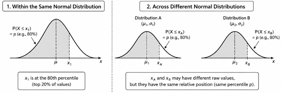
Percentiles and proportions (probabilities) can be used to compare the relative position of an individual value within the same normal distribution or across different normal distributions.
Rather than comparing raw values directly, percentiles and proportions describe how a value ranks relative to the rest of the distribution.
This allows meaningful comparisons even when the distributions have different means or standard deviations.
Definitions
| Term | Definition |
|---|---|
| Percentile | The percentage of observations that are less than or equal to a given value. |
| Proportion | The probability (or decimal) representing the proportion of observations below, above, or between specified values. |
| Relative Position | The location of an observation compared with all other observations in the distribution. |
Using Percentiles to Compare Values
A percentile tells you how a value compares with the rest of the distribution.
For example:
- A student at the 90th percentile scored higher than approximately 90% of all students.
- A patient at the 25th percentile has a measurement greater than approximately 25% of the population.
Even if two values are different, they have the same relative position if they are at the same percentile.
Using Proportions (Probabilities)
Probabilities can also describe relative position.
Examples include:
- \(P(X<70)=0.84\)
- \(P(X>85)=0.10\)
- \(P(60<X<80)=0.65\)
These probabilities represent the proportion of observations that fall below, above, or within a specified interval.
Example 1: Comparing Percentiles
- Student A scored at the 82nd percentile on an AP Statistics exam.
- Student B scored at the 75th percentile on an AP Biology exam.
Comparison
Although the exams are different, Student A performed better relative to other students because the 82nd percentile is higher than the 75th percentile.
Example 2: Comparing Scores from Different Normal Distributions
| Student | Score | Percentile |
|---|---|---|
| A (Math Exam) | 92 | 90th |
| B (Science Exam) | 96 | 85th |
Although Student B earned the higher raw score, Student A has the better relative performance because the 90th percentile is higher than the 85th percentile.
Why Percentiles Are Useful
- Allow comparisons across different normal distributions.
- Describe relative standing rather than raw values.
- Account for differences in means and standard deviations.
- Help compare performances on different tests or measurements.
Important AP Exam Notes
- Percentiles describe an observation’s relative position within a distribution.
- A higher percentile indicates a higher relative standing.
- Raw values from different distributions should not be compared directly.
- Percentiles and probabilities allow meaningful comparisons across different normal distributions.
- The AP Statistics Exam often asks students to interpret a percentile in context.
Common AP Exam Mistakes
| Incorrect | Correct |
|---|---|
| Comparing raw scores from different distributions. | Compare percentiles or relative positions instead. |
| Thinking the 80th percentile means a score of 80. | It means the score is greater than approximately 80% of observations. |
| Assuming equal raw scores always represent equal performance. | Relative performance depends on the distribution. |
Example
Emma scored at the 88th percentile on a college entrance exam.
Noah scored at the 81st percentile on a different standardized exam.
Who performed better relative to the other test takers? Explain.
▶️ Answer / Explanation
Emma performed better relative to the other test takers.
Her score is at the 88th percentile, meaning she scored higher than approximately 88% of the students who took her exam.
Noah scored at the 81st percentile, meaning he scored higher than approximately 81% of the students who took his exam.
Since 88th percentile > 81st percentile, Emma has the higher relative position, even though the two exams may have had different scoring scales.