
2.12.A.1 Sampling Distribution of a Statistic
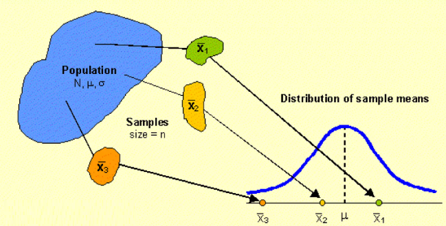
A sampling distribution is the distribution of a statistic calculated from all possible random samples of the same size taken from the same population.
Instead of describing individual observations, a sampling distribution describes how a sample statistic (such as a sample mean or sample proportion) varies from sample to sample.
Definition
A sampling distribution of a statistic is the distribution of values of the statistic for all possible samples of a given size from a given population.
Key Idea
- Every random sample produces a slightly different value of the statistic.
- If we repeatedly take samples of the same size from the same population and calculate the statistic each time, the collection of all those statistic values forms the sampling distribution.
Population vs. Sample vs. Sampling Distribution
| Concept | Description |
|---|---|
| Population | The complete group of individuals or observations being studied. |
| Sample | One subset selected from the population. |
| Statistic | A numerical summary calculated from one sample (such as \(\bar{x}\) or \(\hat{p}\)). |
| Sampling Distribution | The distribution of the statistic from all possible samples of the same size. |
Example 1
Suppose a population consists of the numbers
\(2,\;4,\;6,\;8\)
Randomly select samples of size
\(n=2\)
For every possible sample, calculate the sample mean \(\bar{x}\).
| Sample | Sample Mean \(\bar{x}\) |
|---|---|
| (2,4) | 3 |
| (2,6) | 4 |
| (2,8) | 5 |
| (4,6) | 5 |
| (4,8) | 6 |
| (6,8) | 7 |
The distribution of the values
\(3,\;4,\;5,\;5,\;6,\;7\)
is the sampling distribution of the sample mean.
Example 2
A school has 500 students.
Repeatedly select random samples of 50 students and calculate the average number of hours they study each week.
Each sample produces a different sample mean.
The distribution of all of these sample means is the sampling distribution of the sample mean.
Characteristics of a Sampling Distribution
- It is a distribution of a statistic, not individual observations.
- Every sample must have the same sample size.
- All samples come from the same population.
- The sampling distribution shows how the statistic varies from sample to sample.
Important AP Exam Notes
- A sampling distribution is the distribution of a sample statistic, not the distribution of the original data.
- The statistic may be a sample mean, sample proportion, or another numerical summary.
- Every sample used to construct the sampling distribution must have the same sample size.
- Sampling distributions are used as the foundation for confidence intervals and hypothesis tests.
Common AP Exam Mistakes
| Incorrect | Correct |
|---|---|
| Confusing a population distribution with a sampling distribution. | A sampling distribution is the distribution of a statistic from many samples. |
| Using samples of different sizes. | All samples must have the same size. |
| Thinking a sampling distribution is based on one sample. | It is based on all possible samples (or many repeated samples). |
| Confusing observations with statistics. | A sampling distribution contains statistic values, not individual data values. |
Example
A researcher repeatedly selects random samples of 100 voters from the same population and calculates the sample proportion who support a new policy.
What is the sampling distribution in this situation?
▶️ Answer / Explanation
Each sample produces one sample proportion, \(\hat{p}\).
The distribution of all possible values of \(\hat{p}\) from random samples of 100 voters is the sampling distribution of the sample proportion.
It describes how the sample proportion varies from sample to sample.
2.12.A.2 Simulating a Sampling Distribution
A sampling distribution can be approximated using a simulation instead of collecting every possible sample from a population.
To create the simulation, repeatedly generate a large number of random samples of the same size from the population, calculate the statistic for each sample, and record its value.
The distribution of the recorded statistic values approximates the sampling distribution.
Definition
The sampling distribution of a statistic can be simulated by:
- Assuming the population parameter(s) are known.
- Repeatedly generating many random samples of the same size from the population.
- Calculating the statistic for each sample.
- Recording the statistic.
- Using the collection of statistic values to approximate the sampling distribution.
How a Simulation Works
| Step | Description |
|---|---|
| 1 | Start with a known population or assume known population parameter(s). |
| 2 | Randomly select a sample of fixed size \(n\). |
| 3 | Calculate the statistic (such as \(\bar{x}\) or \(\hat{p}\)). |
| 4 | Repeat thousands of times. |
| 5 | Graph or summarize the recorded statistic values. |
Example 1: Simulating Sample Means
A population has a known mean of 70.
A computer repeatedly selects random samples of
\(n=30\)
students from the population.
For each sample, the sample mean \(\bar{x}\) is calculated and recorded.
After 10,000 samples, the collection of sample means forms an approximation of the sampling distribution of the sample mean.
Example 2: Simulating Sample Proportions
Suppose 60% of voters support a proposal.
A simulation repeatedly selects random samples of
\(n=100\)
voters.
For each sample, the sample proportion \(\hat{p}\) is calculated.
The distribution of the thousands of sample proportions approximates the sampling distribution of \(\hat{p}\).
Why Use Simulations?
- Finding every possible sample is often impossible for large populations.
- Technology can quickly generate thousands of random samples.
- The simulated distribution closely approximates the true sampling distribution.
- Simulations help visualize sampling variability.
Simulation vs. Sampling Distribution
| True Sampling Distribution | Simulated Sampling Distribution |
|---|---|
| Based on all possible samples. | Based on many randomly generated samples. |
| Usually impossible to construct exactly. | Provides an excellent approximation. |
| Theoretical distribution. | Approximate distribution created using technology. |
Important AP Exam Notes
- A simulation repeatedly generates random samples of the same size.
- The statistic is calculated for each sample, not for the entire population.
- The resulting distribution of statistic values approximates the sampling distribution.
- The more simulated samples that are generated, the better the approximation.
- Technology is commonly used to perform thousands of repetitions.
Common AP Exam Mistakes
| Incorrect | Correct |
|---|---|
| Recording every observation from each sample. | Record only the statistic (such as \(\bar{x}\) or \(\hat{p}\)). |
| Changing the sample size during the simulation. | Keep the sample size fixed throughout the simulation. |
| Thinking the simulation produces the exact sampling distribution. | It provides an approximation of the sampling distribution. |
| Using only a few simulated samples. | Thousands of repetitions provide a better approximation. |
Example
A computer repeatedly selects 5,000 random samples of 50 households from a population. For each sample, the sample mean monthly electricity bill is calculated.
Explain how this simulation approximates the sampling distribution of the sample mean.
▶️ Answer / Explanation
Each random sample of 50 households produces one sample mean.
By calculating and recording the sample mean for all 5,000 samples, the resulting distribution of sample means approximates the sampling distribution of the sample mean.
The large number of repetitions makes the approximation close to the true sampling distribution.
2.12.A.3 Randomization Distribution
A randomization distribution is a distribution of a statistic created through simulation by repeatedly randomly reallocating (reassigning) the observed response values to treatment groups.
After each random reallocation, the statistic of interest is calculated and recorded. The collection of these statistic values forms the randomization distribution, which approximates the sampling distribution of the statistic under the assumption that there is no treatment effect.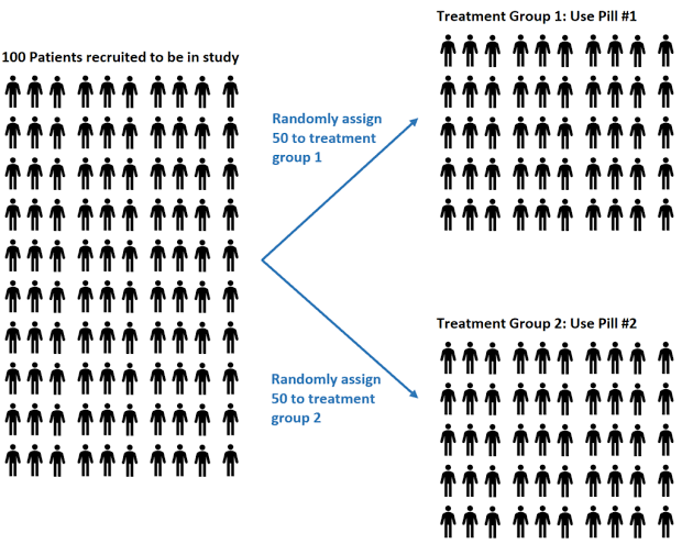
Definition
A randomization distribution is the distribution of a statistic generated by repeatedly:
- Randomly reallocating (reassigning) the response values to treatment groups.
- Calculating the statistic for each reallocation.
- Recording the value of the statistic.
The resulting distribution approximates the sampling distribution of the statistic.
How a Randomization Distribution is Created
| Step | Description |
|---|---|
| 1 | Collect the observed response values. |
| 2 | Randomly reassign the response values to the treatment groups while keeping the group sizes the same. |
| 3 | Calculate the statistic of interest (such as the difference in sample means or proportions). |
| 4 | Repeat the random reassignment thousands of times. |
| 5 | Use the recorded statistics to form the randomization distribution. |
Purpose of a Randomization Distribution
A randomization distribution is used to determine whether an observed statistic is unusual if there is no real difference or treatment effect.
It serves as the basis for estimating a p-value in a hypothesis test.
Example 1: Testing a New Teaching Method
A teacher randomly assigns 30 students to either a new teaching method or the traditional method.
After the experiment, the difference in the average test scores between the two groups is calculated.
To create a randomization distribution:
- The students’ test scores are repeatedly reassigned randomly to the two teaching groups.
- After each reassignment, the difference in sample means is calculated.
- Thousands of simulated differences form the randomization distribution.
Example 2: Medical Experiment
Researchers compare a new medication with a placebo.
Assuming the medication has no effect, the patient outcomes are repeatedly reassigned to the treatment and placebo groups.
The difference in the sample means is calculated for each reassignment.
The resulting distribution is the randomization distribution.
Randomization Distribution vs. Sampling Distribution
| Sampling Distribution | Randomization Distribution |
|---|---|
| Generated by repeatedly taking random samples from a population. | Generated by repeatedly randomly reassigning the observed responses to treatment groups. |
| Describes sampling variability. | Describes the variability expected if there is no treatment effect. |
| Used for estimation and confidence intervals. | Used mainly for hypothesis testing. |
Important AP Exam Notes
- A randomization distribution is created by randomly reallocating (reassigning) the observed response values to treatment groups.
- The sample sizes for each treatment group remain the same during every reassignment.
- Each simulated reassignment produces one value of the statistic.
- The distribution of the simulated statistics approximates the sampling distribution of the statistic under the assumption of no treatment effect.
- Randomization distributions are commonly used to estimate p-values in hypothesis tests.
Common AP Exam Mistakes
| Incorrect | Correct |
|---|---|
| Thinking new data are collected for each simulation. | The original response values are repeatedly reassigned. |
| Changing the sizes of the treatment groups. | Group sizes remain fixed throughout the simulation. |
| Confusing a sampling distribution with a randomization distribution. | A sampling distribution uses repeated samples; a randomization distribution uses repeated reassignments. |
| Assuming a randomization distribution estimates the treatment effect. | It represents what would happen if there were no treatment effect. |
AP Exam Example
A researcher compares the average growth of plants given two different fertilizers. The observed difference in the sample means is 4.2 cm.
To test whether the fertilizers differ in effectiveness, a randomization distribution is created.
Explain how the randomization distribution is generated.
▶️ Answer / Explanation
The observed plant growth measurements are repeatedly randomly reassigned to the two fertilizer groups while keeping the group sizes the same.
For each reassignment, the difference in the sample means is calculated and recorded.
The collection of these simulated differences forms the randomization distribution, which approximates the sampling distribution of the statistic under the assumption that the fertilizers have no difference in effect.
2.12.A.4 Central Limit Theorem (CLT)
The Central Limit Theorem (CLT) is one of the most important concepts in AP Statistics.
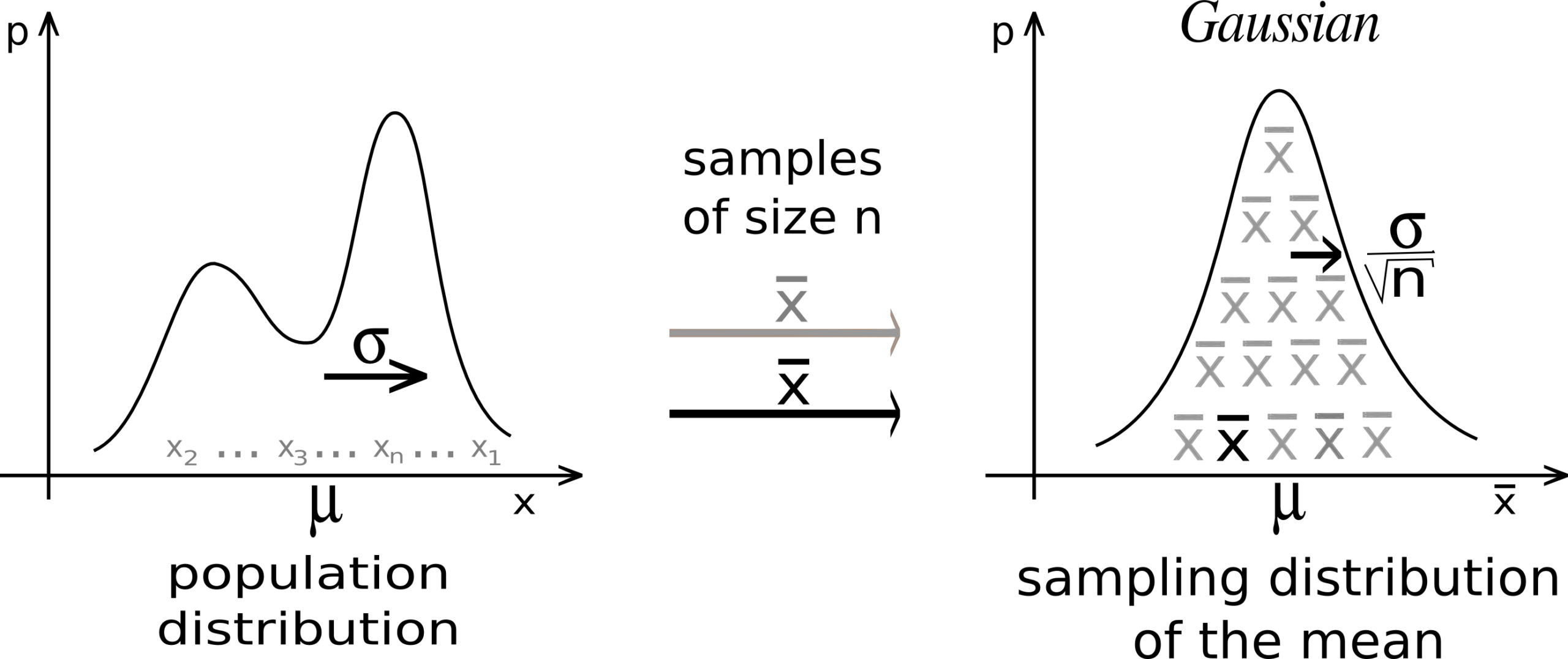
It states that the sampling distribution of the sample mean becomes approximately normal as the sample size increases, regardless of the shape of the population distribution.
This theorem allows statisticians to use the normal distribution for many statistical procedures, even when the original population is not normally distributed.
Definition
The Central Limit Theorem (CLT) states that:
The sampling distribution of the sample mean from a random sample can be approximated by a normal distribution. The larger the sample size, the better the normal approximation.
Key Ideas of the Central Limit Theorem
- The CLT applies to the sampling distribution of the sample mean, not the population distribution.
- As the sample size increases, the sampling distribution becomes more nearly normal.
- If the population is already normally distributed, the sampling distribution of the sample mean is normal for any sample size.
- If the population is not normal, larger sample sizes improve the normal approximation.
Effect of Sample Size
| Sample Size | Shape of the Sampling Distribution |
|---|---|
| Small | May resemble the population distribution. |
| Moderate | Begins to look more normal. |
| Large (typically \(n\ge30\)) | Usually well approximated by a normal distribution. |
Note: The guideline \(n\ge30\) is commonly used in AP Statistics, although the required sample size depends on how skewed the population distribution is.
Example 1: Normally Distributed Population
Suppose the heights of adult women are normally distributed.
If random samples of
\(n=10\)
are selected, the sampling distribution of the sample mean is also normal.
This is true because the original population is normal.
Example 2: Skewed Population
Suppose household incomes are strongly right-skewed.
If random samples of
\(n=100\)
are selected, the sampling distribution of the sample mean will be approximately normal, even though the population itself is not normal.
This occurs because of the Central Limit Theorem.
Population Distribution vs. Sampling Distribution
| Population Distribution | Sampling Distribution of \(\bar{x}\) |
|---|---|
| Distribution of individual observations. | Distribution of sample means. |
| Can have almost any shape. | Becomes approximately normal as sample size increases. |
| Does not change. | Depends on the sample size. |
Why the Central Limit Theorem Matters
- It allows the use of normal probability calculations for sample means.
- It is the foundation for confidence intervals and hypothesis tests involving means.
- It explains why many statistical procedures work even when the population is not normally distributed.
Important AP Exam Notes
- The Central Limit Theorem applies to the sampling distribution of the sample mean, not the population distribution.
- As the sample size increases, the sampling distribution becomes more nearly normal.
- If the population is already normal, the sampling distribution is normal for any sample size.
- For non-normal populations, larger sample sizes (commonly \(n\ge30\)) generally provide a good normal approximation.
- The CLT is used to justify many inference procedures involving population means.
Common AP Exam Mistakes
| Incorrect | Correct |
|---|---|
| Thinking the CLT makes the population normal. | The CLT applies to the sampling distribution, not the population. |
| Confusing individual observations with sample means. | The CLT describes the distribution of sample means. |
| Assuming the CLT requires a normal population. | A normal population is not required when the sample size is sufficiently large. |
| Believing \(n=30\) always guarantees a perfect normal distribution. | \(n\ge30\) is a guideline; highly skewed populations may require larger samples. |
Example
A population of household incomes is strongly right-skewed.
A researcher repeatedly selects random samples of 100 households and calculates the sample mean income.
Describe the shape of the sampling distribution of the sample mean and explain why.
▶️ Answer / Explanation
Although the population distribution is strongly right-skewed, the sampling distribution of the sample mean will be approximately normal.
This is a result of the Central Limit Theorem, which states that as the sample size becomes large, the sampling distribution of the sample mean approaches a normal distribution.