Calculate Statistics for Two Categorical Variables
When we have two categorical variables, we summarize and analyze their relationship using: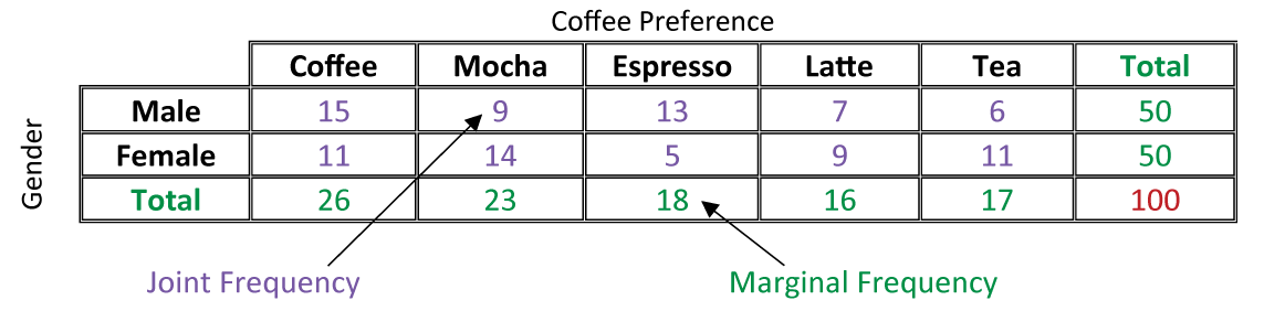
- Counts in a two-way (contingency) table (joint frequencies)
- Marginal, joint, and conditional relative frequencies
- Measures of association for 2×2 tables: relative risk and odds ratio
- Formal inference: the chi-square test of independence (with expected counts and residuals)
- Measure of effect size: Cramér’s V
Common formulas
- Joint relative frequency: \( \text{Joint RF} = \dfrac{\text{cell count}}{n} \).
- Marginal relative frequency: \( \text{Marginal RF} = \dfrac{\text{row or column total}}{n} \).
- Conditional relative frequency: \( P(A \mid B) = \dfrac{\text{count of (A and B)}}{\text{total in category }B} \).
Example
A survey of 100 students recorded Gender (Male/Female) and whether they prefer sports (Yes/No). The observed counts:
| Sports: Yes | Sports: No | Total | |
|---|---|---|---|
| Male | 30 | 10 | 40 |
| Female | 20 | 40 | 60 |
| Total | 50 | 50 | 100 |
▶️ Answer / Explanation
Step 1: Joint relative frequencies
- Male & Yes: \( \dfrac{30}{100} = 0.30 \)
- Female & No: \( \dfrac{40}{100} = 0.40 \)
Step 2: Conditional relative frequencies
- \( P(\text{Yes} \mid \text{Male}) = \dfrac{30}{40} = 0.75 \)
- \( P(\text{Yes} \mid \text{Female}) = \dfrac{20}{60} \approx 0.33 \)
Because 0.75 ≠ 0.33, the two variables are associated.
Compare Statistics for Two Categorical Variables
In a two-way (contingency) table, we can summarize relationships using marginal relative frequencies and conditional relative frequencies. These allow us to compare groups and determine whether the variables appear to be associated.
Marginal Relative Frequency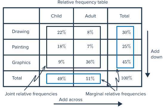
Computed from the row totals or column totals of a two-way table.
- Formula: \( \text{Marginal RF} = \dfrac{\text{Row (or Column) Total}}{\text{Grand Total}} \).
- Represents the overall distribution of one variable regardless of the other variable.
Conditional Relative Frequency
Calculated within a specific row or column.
- Formula: \( P(A \mid B) = \dfrac{\text{Cell Count for (A and B)}}{\text{Row or Column Total for } B} \).
- Represents the distribution of one variable given a category of the other variable.
Comparison
- Marginal RF gives overall proportions (ignores the second variable).
- Conditional RF compares groups within categories (helps identify possible association).
- If conditional RFs are very different across groups, the variables are likely associated.
Example
A survey of 120 students recorded Class Level (Freshman/Senior) and whether they prefer pop music (Yes/No). Results are shown:
| Pop: Yes | Pop: No | Total | |
|---|---|---|---|
| Freshman | 40 | 20 | 60 |
| Senior | 15 | 45 | 60 |
| Total | 55 | 65 | 120 |
▶️ Answer / Explanation
Step 1: Marginal Relative Frequencies
- Freshmen: \( \dfrac{60}{120} = 0.50 \).
- Seniors: \( \dfrac{60}{120} = 0.50 \).
- Pop Yes: \( \dfrac{55}{120} \approx 0.458 \).
- Pop No: \( \dfrac{65}{120} \approx 0.542 \).
Step 2: Conditional Relative Frequencies
- Among Freshmen: \( P(\text{Yes} \mid \text{Freshman}) = \dfrac{40}{60} \approx 0.667 \).
- Among Seniors: \( P(\text{Yes} \mid \text{Senior}) = \dfrac{15}{60} = 0.25 \).
Step 3: Interpretation
The marginal RFs show that 45.8% of students overall prefer pop. But conditional RFs show a much higher proportion of Freshmen (≈66.7%) than Seniors (25%). Since these proportions differ substantially, music preference appears to be associated with class level.